Shared posts

17 Feb 08:53

The useful functions for modern OpenGL 4.4 programming

If anything, at least Mantle created some discussions about graphics API but it remains that I believe it's a waste of AMD engineering resources that could have benefit their OpenGL drivers for example.

Looking at the published list of Mantle functions, Mantle API looks really thin compared to OpenGL API for example. However, Mantle targets only AMD Southern Islands onward, while OpenGL 4.4 core profile targets all OpenGL 3 / Direct3D 10 and OpenGL 4 / Direct3D 11 GPUs. If we consider OpenGL 4.4 compatibility profile, then the API covers all GPUs even made.

Let's compare what we can compare. What if we want to write a Modern OpenGL program for AMD Southern Islands and NVIDIA Kepler only. Then we only need a tiny subset of the OpenGL API that I have listed below.

It still appears that Mantle requires less functions. With a closer look we see that Mantle use state objects to group rasterizer, viewport, depth test states. State objects are a idea because every hardware vendor would want different packing but also because every single OpenGL program would use different packing. To write an efficient OpenGL renderer we need to consider the update frequences and move every operations at the lower update rate possible. Packing states is requiring to update more often states that should not have change hence adding CPU overhead. So no thank you but I prefer to have no state object. However, what worked for me in the past (about 2007) was to use display lists to create immutable state objects that matched my program needs. I don't think I want to go this way in 2014.

So OpenGL has evolved, "revolution through evolution". If we really want to write low overhead OpenGL programs, we can. If that's not the case right now, my opinion is that the industry didn't put the effort in it because it has higher priority issues to resolve, essentially production issues which include supporting old consoles (PS3 and XBox, OpenGL 2.1 / Direct3D 9 hardware), cross compiling shaders, the development of mobile and the rise of WebGL.

Reflexion API (only for tools developers):
14 Feb 13:33

Functional Data Structures and Concurrency in C++

by Bartosz Milewski
In my previous blog posts I described C++ implementations of two basic functional data structures: a persistent list and a persistent red-black tree. I made an argument that persistent data structures are good for concurrency because of their immutability. In this post I will explain in much more detail the role of immutability in concurrent […]
14 Feb 13:33

Functional Data Structures in C++: Trees

by Bartosz Milewski
Persistent trees are more interesting than persistent lists, which were the topic of my previous blog. In this installment I will concentrate on binary search trees. Such trees store values that can be compared to each other (they support total ordering). Such trees may be used to implement sets, multisets, or associated arrays. Here I […]
14 Feb 13:33

Functional Data Structures in C++: Lists

by Bartosz Milewski
“Data structures in functional languages are immutable.” What?! How can you write programs if you can’t mutate data? To an imperative programmer this sounds like anathema. “Are you telling me that I can’t change a value stored in a vector, delete a node in a tree, or push an element on a stack?” Well, yes […]
10 Feb 08:35

Porting from Windows to Linux, part 1

by Anteru

Hi and welcome to a blog series about how to port graphics applications from Windows to Linux. The series will have three parts: Today, in the first part, we’ll be looking at prerequisites for porting. These are things you can do any time to facilitate porting later on, while still working on Windows exclusively. In the second part, the actual porting work will be done, and in the last part, I’ll talk a bit about the finishing touches, rough edges, and how to keep everything working. All of this is based on my experience with porting my research framework; which is a medium-sized project (~ 180 kLoC) that supports Linux, Windows and Mac OS X.

However, before we start, let’s assess the state of the project before the porting begins. For this series, I assume you have a Visual Studio based solution written in C++, with Direct3D being used for graphics. Your primary development environment is Visual Studio, and you haven’t developed for Linux before. You’re now at the point where you want to add Linux support to your application while keeping Windows intact — so we’re not talking about a rushed conversion from Windows to Linux, but of a new port of your application which will be maintained and supported alongside the Windows version.

Prerequisites

Let’s start by sorting out the obvious stuff: Your need a source control solution which will work on Linux. If your project is stored in TFS, now is the time to export everything to your favourite portable source control. If you are not sure what to choose, take Mercurial, which comes with a nice UI for all platforms.

Next, check all your dependencies. If you rely on WIC for image loading, you’ll have to find a portable solution first. In my experience, it’s usually easier to have the same code running on Windows and Linux later on than having a dedicated path for each OS. In my project, I wrapped the low-level libraries like libpng or libjpg directly instead of using a larger image library.

Now is also the time to write tests. You’ll need to be able to quickly verify that everything is working again. If you haven’t written any automated tests yet, this is the moment to start. You’ll mostly need functional tests, for instance, for disk I/O, so focus on those first. I say mostly functional tests, as unit tests tend to be OS agnostic. In my framework, unit tests cover low-level OS facilities like threads and memory allocators, while everything else, including graphics, is covered by functional tests.

For testing, I can highly recommend Google Test. It’s not designed for functional tests right away, but it’s very easy to write a wrapper around a Google Test enabled project for functional testing. My wrapper is written in Python and sets up a new folder for each functional test, executes each test in a new process and gathers all results.

Finally, if you have any build tools, make sure that those are portable now. I used to write them in C# when it was really new, but since a few years, I use only Python for build tools. Python code tends to be easy to maintain and it requires no build process whatsoever, making it ideally suited for build system infrastructure. Which brings us to the most important issue, the build sytem.

Build system

If you are using Visual Studio (or MSBuild from the command line), stop right now and start porting it to a portable build system. While in theory, MSBuild is portable to Linux using xbuild, in practice, you’ll still want to have a build system which is developed on all three platforms and used for large code bases. I have tried a bunch of them and finally settled with CMake. It uses an arcane scripting language, but it works, and it works reliably on Windows, Linux, and Mac OS X.

Porting from Visual Studio to CMake might seem like a huge effort at first, but it’ll make the transition to Linux much easier later on. The good thing about CMake is that it works perfectly on Windows and it produces Visual Studio project files, so your existing Windows developer experience remains the same. The only difference is that adding new source files now requires you to edit a text file instead of using the IDE directly, but that’s about it.

While writing your CMake files, here’s a few things you should double-check:

  • Are your path names case-sensitive? Windows doesn’t care, but on Linux, your include directory won’t be found if you mess up paths.
  • Are you setting compiler flags directly? Check if CMake already sets them for you before adding a huge list of compiler flags manually.
  • Are your dependencies correctly set up? With Visual Studio, it’s possible to not define all dependencies correctly and still get a correct build; while other build tools will choke on it. Use the graph output of CMake to visualize the dependencies and double check both the build order, and the individual project dependencies.

With CMake, you should also take advantage of the “Find” mechanism for dependencies. On Linux, nearly all dependencies are available as system libraries, serviced by the package manager, so it definitely makes sense to link against the system version of a dependency if it is recent enough.

The end result of this step should be exactly the same binaries as before, but using CMake as the build system instead of storing the solutions directly in source control. Once this is done, we can start looking at the code.

Clean code

Did you ever #include system headers like <windows.h> in your code? Use system types like DWORD? Now is the time to clean up and to isolate these things. You want to achieve two goals here:

  • Remove system includes from headers as much as possible.
  • Remove any Visual C++ specific code.

System headers should be only included in source files, if possible. If not, you should isolate the classes/functions and provide generic wrappers around them. For instance, if you have a class for handling files, you can either use the PIMPL idiom or just derive a Windows-specific class from it. The second solution is usually simpler if your file class is already derived from somewhere (a generic stream interface, for instance.) Even if not, we’re wrapping an extremely slow operating system function here (file reads will typically hit the disk), so the cost of a virtual function call won’t matter in practice.

To get rid of Visual C++ specific code, turn on all warnings and treat them as errors. There are a bunch of bogus warnings you can disable (I’ve blogged about them previously), but everything else should get fixed now. In particular, you don’t want any Visual C++ specific extensions enabled in headers. The reason why you want all warnings to be fixed is that on Linux, you’ll be getting hundreds of compile errors and warnings at first, and the less these are swamped by issues that are also present on Windows, the better.

While cleaning up, you should pay special attention to integer sizes. Windows uses 32-bit longs in 64-bit mode, Linux defaults to 64-bit longs. To avoid any confusion, I simply use 64-bit integers when it comes to memory sizes.

The better you clean up your code, the less work you’ll have to spend later during porting. The goal here should be to get everything to build on Windows, with platform specific files identified and isolated.

So much for today! Next week, we’ll look at how to get rid of Direct3D and how to start bringing up the code base on Linux. Stay tuned!

28 Jan 16:24

Never Again in Graphics: Unforgivable graphic curses.

by DEADC0DE
Well known, zero cost things that still are ignored too often.

Do them. On -any- platform, even mobile.

Please.
  • Lack of self-occlusion. Pre-compute aperture cones on every mesh and bend the normalmap normals, change specular occlusion maps and roughness to fit the aperture cone. The only case where this doesn't apply is for animated models (i.e. characters), but even there baking in "t-pose" isn't silly (makes total sense for faces for example), maybe with some hand-authored adjustments.
  • Non-premultiplied alpha.
  • Wrong Alpha-key mipmaps computed via box (or regular image) filters.
  • Specular aliasing (i.e. not using Toksvig or similar methods).
  • Analytic, constant emission point/spot lights.
  • Halos around DOF filters. Weight your samples! Maybe only on low-end mobile, if you just do a blur and blend, it might be understandable that you can't access the depth buffer to compute the weights during the blur...
  • Cartoon-shading-like SSAO edges. Weight your samples! Even if for some reason you have to do SSAO over the final image (baaaad), at least color it, use some non-linear blending! Ah, and skew that f*cking SSAO "up", most light comes from sky or ceiling, skewing the filter upwards (shadows downwards) is more realistic than having them around objects. AND don't multiply it on top of the final shading! If you have to do so (because you don't have a full depth prepass) at least do some better blending than straight multiply!
  • 2D Water ripples on meshes. This is the poster child of all the effects that can be done, but not quite right. Either you can do something -well enough- or -do not do it-. Tone it down! Find alternatives. Look at reference footage!
  • Color channel clamping (after lighting), i.e. lack of tonemapping. Basic Reinhard is cheap, even on shaders on "current-gen" (if you're forced to output to a 8bit buffer... and don't care that alpha won't blend "right").
  • Simple depth-based fog. At least have a ground! And change the fog based on sun dot view. Even if it's constant per frame, computed on the CPU.
If you can think of more that should go in the list, use the comments section!
28 Jan 16:24

In the next-generation everything will be data (maybe)

by DEADC0DE
I've just finished sketching a slide deck on data... stuff. And I remembered I had a half-finished post on my blog tangentially related to that, so I guess it's time to finish it. Oh. Oh. I didn't remember it was rambling so much. Brace yourself...

Rant on technology and games.
Computers, computing is truly revolutionary. Every technological advance has been incredible, enabling us to deal with problems, to work, to express ourselves in ways we could have never imagined. It's fascinating, and it's one of the things that drew me to computer science to begin with.

Why am I writing this? Games are high-tech, we know that, is this really the audience for such a talk? Well. Truth is, really, we aren't that much. Now I know, the grass is always greener and everything, but really in the past decade or so technology surprised me yet again and turned things over their heels. Let's face it, the web won. Languages come and go, code is edited live, methodologies evolve, psychology, biometrics, a lot of cool happens there, innovation. It's a thriving science. Well, web and trading (but let's not talk of evil stuff here for now) and maybe some other fields, you get the point.

Now, I think I even know why: algorithms make money in these fields. Shaving milliseconds can mark the success or death of a service. I am, supposedly, in one of the most technical subfields of videogame programming: rendering. Yet it's truly hard to say whether an innovation I might produce does make more money on a shipped title. It's even debatable what kind of dent in sales better visuals as a whole do make. We're quite far removed, maybe a necessary condition, at best, but almost always not sufficient.

Now, actually I don't want to put our field down that much. We're still cool. Technology still matters and I'm not going to quit my job anytime soon and I enjoy the technological part of it as well as the other parts. But, there's space to learn, and I think it's time to start looking at things with a different perspective...

An odd computing trick that rendering engineers don't want you to know.
Sometimes, working on games, engineers compete on resources. Rendering takes most, and the odd thing is we can still complain about how much animation, UI, AI, and audio take. All your CPU are belong to us

To a degree we are right, see for example what happens when a new console comes out. Rendering takes it all (even struggling), gameplay usually fits, happy to have more memory sitting around unused. We are good at using the hardware, the more hardware, the more rendering will do. And then everybody complains that rendering was already "good enough" and that games don't change and animation is the issue and so on.

Rendering in other words, scales. SIMD? More threads? GPUs? We eat them all... Why? Well, because we know about data! We're all about data. 

Don't tell people around, but really, at its best rendering is a few simple kernels that go through data wrapped hopefully in an interface that doesn't upset artists too much. We take a scene of several thousands of objects and we find the visible ones from a few different points of view. Then we sort and them and send everything to the GPU. 

Often the most complex of all this is loading and managing the data and everything that happens around the per-frame code. The GPU? Oh, there things get even more about the data! It goes through millions of triangles, transforms them to place them on screen and then yet again finds the visible ones. These generate pixels that are even more data, for which we need to determine a color. Or roughly something like that.

The amount of data we filter through our few code "kernels" is staggering, so it's we devote a lot of care to them. 

Arguably many "unsuccessful" visuals are due to trying to do more than it's worth doing or it's possible to do well. Caring too much for the number of features instead of specializing on a few very well executed data paths. You could even say that Carmack has been very good at this kind of specialization and that made his technology have quite the successful legacy it has.

Complexity and cost.
Ok all fine, but why should we (and by we I'm imagining "non-rendering" engineers) care? Yes, "gameplay" code is more "logic" than "data", that's maybe the nature of it and there's nothing wrong with it. Also wasn't code a compressed form of data anyhow?

True, but does it have to be this way? Let's start talking about why it maybe shouldn't. Complexity. The least code, the best. And we're really at a point where everybody is scared about complexity, our current answer is tools, as in, doing the same thing, with a different interface. 

Visual programming? Now we're about data right? Because it's not code in a text editor, it's something else... Sprinkle some XML scripting language and you're data-oriented.
So animation becomes state machines and blend trees. AI becomes scripts, behaviour trees and boxes you connect together. Shaders and materials? More boxes!

An odd middle ground, really we didn't fundamentally change the ways things are computed, just wrapped them changing the syntax a bit, not the semantic. Sometimes you can win something from a better syntax, most of these visual tools don't as now we have to maintain a larger codebase (a runtime, a custom script interpreter, some graphical interfaces over them...) that expresses at best the same capabilities as pure code. 
We gain a bit when we have to iterate over the same kind of logic (because C++ is hard, slow, and so on) but we lose when we have to add completely new functionalities (that require modifications to the "native" runtime and to be propagated through tools).

This is not the kind of "data-driven" computation I'll be talking about and it is an enormous source of complexity.

Data that drives.
Data comes in two main flavours, sort of orthogonal to each other: acquisition and simulation. Acquired data is often to expensive to store, and needs to be compressed in some ways. Simulated (generated) data is often expensive to compute, and we can offset that with storage (precomputation). 
Things get even more interesting when you chain both i.e. you precompute simulated data and then learn/compress models out of it, or you use acquired data to instruct simulated models, and so on.

Let's take animation. We have data, lots of it, motion capture is the de-facto standard for videogame animation. Yet, all we do it to clean it up, manually keyframe a bit, then manually chop, split, devise a logic, connect pieces together, build huge graphs dictating when a given clip can transition into another, how two clips can blend together and so on. For hundreds of such clips, states and so forth. 
Acquisition gets manually ground into the runtime, and simulation is mostly relegated to minor aesthetic details. Cloth, hair, ragdolls. When you're lucky collisions and reactions to them.

Can we use the original data more? Filter, learn models. If we know what a character should do, then can we search for the most "fitting" data we have automatically, an animation that has a pose that conserves what matters (position, momentum) and goes where we want to go... Yes, it turns out, we can. 
Now, this is just an example, and I can't even begin to scratch the surface of the actual techniques, so I won't. If you do animation and this is new to you, start from Popovic (continuos character control with low dimensional embeddings is to the date the most advanced of his "motion learned from data" approaches, even if kNN based solutions or synthesis of motion trees might be most practical today) and explore from there.

All of this is not even completely unexplored, AAA titles are shipping with methods that replace hardcoding with data and simulation. An example is the learning-based method employed for the animation of crowds in Hitman:Absolution
I had the pleasure of working from many years with the sports group at EA, which surely knows animation and AI very well, shipping what was at the date I think one of the very few AAA titles with a completely learning-based AI, Fight Night Round 4
The work of Simon Clavet (responsible for the animation of Assissin's Creed 3) is another great example, this time towards the simulation end of the spectrum.

What I'd really wish is to see if we can actually use all the computing power we have to make better games, via a technological revolution. We're going to really enter a "next generation" of gaming if we learn more on what we can do with data. In the end it's computer science, actually all there is to it. Which is both thrilling and scary, it means we have to be better at it, and how much there is to learn.
    • Data acquisition:  filtering, signal processing, but also understanding what matters which means metrics.
      • Animation works with a lot of acquisition. Gameplay acquires data too, telemetry but also some studios experiment with biometrics and other forms of user testing. Rendering is just barely starting with data (e.g. HDR images, probes, BRDF measurements).
      • Measures and errors. Still have lots to understand about Perception and Psychology (what matters! artists right now are our main guidance, which is not bad, listen to them). Often we don't really know what errors we have in the data, quantitatively.
      • Simulation, Visualization, Exploration.
    • Representation, which is huge, everything really is compression, quite literally as code is compressed data, we know, but the field is huge. Learning really is compression too.
    • Runtime, parallel algorithms and GPUs.
      • This is what rendering gets done well today, even if mostly on artist-made data.
      • Gather (Reduce) / Scatter / Transform (Map)
      • For state machines (Animation, AI) a good framework is to think about search and classification. What is the best behaviour in my database for this situation? Given a stage, can I create a classification function that maps to outcomes? And so on.
    In the end it's all a play of shifting complexity from authoring to number crunching. We'll see.
    20 Jan 13:03

    Tech Feature: SSAO and Temporal Blur

    by Peter

    Screen space ambient occlusion (SSAO) is the standard solution for approximating ambient occlusion in video games. Ambient occlusion is used to represent how exposed each point is to the indirect lighting from the scene. Direct lightingis light emitted from a light source, such as a lamp or a fire. The direct light then illuminates objects in the scene. These illuminated objects make up the indirect lighting. Making each object in the scene cast indirect lighting is very expensive. Ambient occlusion is a way to approximate this by using a light source with constant color and information from nearby geometry to determine how dark a part of an object should be. The idea behind SSAO is to get geometry information from the depth buffer.

    There are many publicised algorithms for high quality SSAO. This tech feature will instead focus on improvements that can be made after the SSAO has been generated.


    SSAO Algorithm
    SOMA uses a fast and straightforward algorithm for generating medium frequency AO. The algorithm runs at half resolution which greatly increases the performance. Running at half resolution doesn’t reduce the quality by much, since the final result is blurred.

    For each pixel on the screen, the shader calculates the position of the pixel in view space and then compares that position with the view space position of nearby pixels. How occluded the pixel gets is based on how close the points are to each other and if the nearby point is in front of the surface normal. The occlusion for each nearby pixel is then added together for the final result. 

    SOMA uses a radius of 1.5m to look for nearby points that might occlude. Sampling points that are outside of the 1.5m range is a waste of resources, since they will not contribute to the AO. Our algorithm samples 16 points in a growing circle around the main pixel. The size of the circle is determined by how close the main pixel is to the camera and how large the search radius is. For pixels that are far away from the camera, a radius of just a few pixels can be used. The closer the point gets to the camera the more the circle grows - it can grow up to half a screen. Using only 16 samples to select from half a screen of pixels results in a grainy result that flickers when the camera is moving.
    Grainy result from the SSAO algorithm
    Bilateral Blur
    Blurring can be used to remove the grainy look of the SSAO. Blur combines the value of a large number of neighboring pixels. The further away a neighboring pixel is, the less the impact it will have on the final result. Blur is run in two passes, first in the horizontal direction and then in the vertical direction.

    The issue with blurring SSAO this way quickly becomes apparent. AO from different geometry leaks between boundaries causing a bright halo around objects. Bilateral weighting can be used to fix the leaks between objects. It works by comparing the depth of the main pixel to the depth of the neighboring pixel. If the distance between the depth of the main and the neighbor is outside of a limit the pixel will be skipped. In SOMA this limit is set to 2cm.
    To get good-looking blur the number of neighboring pixels to sample needs to be large. Getting rid of the grainy artifacts requires over 17x17 pixels to be sampled at full resolution.

    Temporal Filtering 
    Temporal Filtering is a method for reducing the flickering caused by the low number of samples. The result from the previous frame is blended with the current frameto create smooth transitions. Blending the images directly would lead to a motion-blur-like effect. Temporal Filtering removes the motion blur effect by reverse reprojecting the view space position of a pixel to the view space position it had the previous frame and then using that to sample the result. The SSAO algorithm runs on screen space data but AO is applied on world geometry. An object that is visible in one frame may not be seen in the next frame, either because it has moved or because the view has been blocked by another object. When this happens the result from the previous frame has to be discarded. The distance between the points in world space determines how much of the result from the previous frame should be used.

    Explanation of Reverse Reprojection used in Frostbite 2 [2]
    Temporal Filtering introduces a new artifact. When dynamic objects move close to static objects they leave a trail of AO behind. Frostbite 2’s implementation of Temporal Filtering solves this by disabling the Temporal Filter for stable surfaces that don’t get flickering artifacts. I found another way to remove the trailing while keeping Temporal Filter for all pixels.


    Shows the trailing effect that happens when a dynamic object is moved. The Temporal Blur algorithm is then applied and most of the trailing is removed.

    Temporal Blur 

    (A) Implementation of Temporal Filtered SSAO (B) Temporal Blur implementation 
    I came up with a new way to use Temporal Filtering when trying to remove the trailing artifacts. By combining two passes of cheap blur with Temporal Filtering all flickering and grainy artifacts can be removed without leaving any trailing. 

    When the SSAO has been rendered, a cheap 5x5 bilateral blur pass is run on the result. Then the blurred result from the previous frame is applied using Temporal Filtering. A 5x5 bilateral blur is then applied to the image. In addition to using geometry data to calculate the blending amount for the Temporal Filtering the difference in SSAO between the frames is used, removing all trailing artifacts. 

    Applying a blur before and after the Temporal Filtering and using the blurred image from the previous frame results in a very smooth image that becomes more blurred for each frame, it also removes any flickering. Even a 5x5 blur will cause the resulting image to look as smooth as a 64x64 blur after a few frames.

    Because the image gets so smooth the upsampling can be moved to after the blur. This leads to Temporal Blur being faster, since running four 5x5 blur passes in half resolution is faster than running two 17x17 passes in full resolution. 

    Upsampling
    All of the previous steps are performed in half resolution. To get the final result it has to be scaled up to full resolution. Stretching the half resolution image to twice its size will not look good. Near the edges of geometry there will be visible bleeding; non-occluded objects will have a bright pixel halo around them. This can be solved using the same idea as the bilateral blurring. Normal linear filtering is combined with a weight calculated by comparing the distance in depth between the main pixel and the depth value of the four closest half resolution pixels.

    Summary 
    Combining SSAO with the Temporal Blur algorithm produces high quality results for a large search radius at a low cost. The total cost of the algoritm is 1.1ms (1920x1080 AMD 5870). This is more than twice as fast as a normal SSAO implementation.

    SOMA uses high frequency AO baked into the diffuse texture in addition to the medium frequency AO generated by the SSAO.

    Temporal Blur could be used to improve many other post effects that need to produce smooth-looking results.

    Ambient Occlusion is only one part of the rendering pipeline, and it should be combined with other lighting techniques to give the final look.


    References
    1. http://gfx.cs.princeton.edu/pubs/Nehab_2007_ARS/NehEtAl07.pdf 
    2. http://dice.se/wp-content/uploads/GDC12_Stable_SSAO_In_BF3_With_STF.pdf 

     // SSAO Main loop

    //Scale the radius based on how close to the camera it is
     float fStepSize = afStepSizeMax * afRadius / vPos.z;
     float fStepSizePart = 0.5 * fStepSize / ((2 + 16.0));    

     for(float d = 0.0; d < 16.0; d+=4.0)
     {
            //////////////
            // Sample four points at the same time
            vec4 vOffset = (d + vec4(2, 3, 4, 5))* fStepSizePart;
            
            //////////////////////
            // Rotate the samples
            vec2 vUV1 = mtxRot * vUV0;
            vUV0 = mtxRot * vUV1;

            vec3 vDelta0 = GetViewPosition(gl_FragCoord.xy + vUV1 * vOffset.x) - vPos;
            vec3 vDelta1 = GetViewPosition(gl_FragCoord.xy - vUV1 * vOffset.y) - vPos;
            vec3 vDelta2 = GetViewPosition(gl_FragCoord.xy + vUV0 * vOffset.z) - vPos;
            vec3 vDelta3 = GetViewPosition(gl_FragCoord.xy - vUV0 * vOffset.w) - vPos;

            vec4 vDistanceSqr = vec4(dot(vDelta0, vDelta0),
                                     dot(vDelta1, vDelta1),
                                     dot(vDelta2, vDelta2),
                                     dot(vDelta3, vDelta3));

            vec4 vInvertedLength = inversesqrt(vDistanceSqr);

            vec4 vFalloff = vec4(1.0) + vDistanceSqr * vInvertedLength * fNegInvRadius;

            vec4 vAngle = vec4(dot(vNormal, vDelta0),
                                dot(vNormal, vDelta1),
                                dot(vNormal, vDelta2),
                                dot(vNormal, vDelta3)) * vInvertedLength;


            ////////////////////
            // Calculates the sum based on the angle to the normal and distance from point
            fAO += dot(max(vec4(0.0), vAngle), max(vec4(0.0), vFalloff));
    }

    //////////////////////////////////
    // Get the final AO by multiplying by number of samples
    fAO = max(0, 1.0 - fAO / 16.0);

    ------------------------------------------------------------------------------ 

    // Upsample Code
     
    vec2 vClosest = floor(gl_FragCoord.xy / 2.0);
    vec2 vBilinearWeight = vec2(1.0) - fract(gl_FragCoord.xy / 2.0);

    float fTotalAO = 0.0;
    float fTotalWeight = 0.0;

    for(float x = 0.0; x < 2.0; ++x)
    for(float y = 0.0; y < 2.0; ++y)
    {
           // Sample depth (stored in meters) and AO for the half resolution 
           float fSampleDepth = textureRect(aHalfResDepth, vClosest + vec2(x,y));
           float fSampleAO = textureRect(aHalfResAO, vClosest + vec2(x,y));

           // Calculate bilinear weight
           float fBilinearWeight = (x-vBilinearWeight .x) * (y-vBilinearWeight .y);
           // Calculate upsample weight based on how close the depth is to the main depth
           float fUpsampleWeight = max(0.00001, 0.1 - abs(fSampleDepth – fMainDepth)) * 30.0;

           // Apply weight and add to total sum
           fTotalAO += (fBilinearWeight + fUpsampleWeight) * fSampleAO;
           fTotalWeight += (fBilinearWeight + fUpsampleWeight);
    }

    // Divide by total sum to get final AO
    float fAO = fTotalAO / fTotalWeight;

    -------------------------------------------------------------------------------------

    // Temporal Blur Code

    //////////////////
    // Get current frame depth and AO
    vec2 vScreenPos = floor(gl_FragCoord.xy) + vec2(0.5);
    float fAO = textureRect(aHalfResAO, vScreenPos.xy);
    float fMainDepth = textureRect(aHalfResDepth, vScreenPos.xy);   

    //////////////////
    // Convert to view space position
    vec3 vPos = ScreenCoordToViewPos(vScreenPos, fMainDepth);

    /////////////////////////
    // Convert the current view position to the view position it 
    // would represent the last frame and get the screen coords
    vPos = (a_mtxPrevFrameView * (a_mtxViewInv * vec4(vPos, 1.0))).xyz;

    vec2 vTemporalCoords = ViewPosToScreenCoord(vPos);
           
    //////////////
    // Get the AO from the last frame
    float fPrevFrameAO = textureRect(aPrevFrameAO, vTemporalCoords.xy);
    float fPrevFrameDepth = textureRect(aPrevFrameDepth, vTemporalCoords.xy);

    /////////////////
    // Get to view space position of temporal coords
    vec3 vTemporalPos = ScreenCoordToViewPos(vTemporalCoords.xy, fPrevFrameDepth);
           
    ///////
    // Get weight based on distance to last frame position (removes ghosting artifact)
    float fWeight = distance(vTemporalPos, vPos) * 9.0;

    ////////////////////////////////
    // And weight based on how different the amount of AO is (removes trailing artifact)
    // Only works if both fAO and fPrevFrameAO is blurred
    fWeight += abs(fPrevFrameAO - fAO ) * 5.0;

    ////////////////
    // Clamp to make sure atleast 1.0 / FPS of a frame is blended
    fWeight = clamp(fWeight, afFrameTime, 1.0);       
    fAO = mix(fPrevFrameAO , fAO , fWeight);
       
    ------------------------------------------------------------------------------


    20 Jan 13:02

    Link collection of using spherical Gaussian approximation for specular shading in games

    by hanecci
    08 Jan 13:01

    Heap Inspector 1.4 is out!

    by admin

    Over the past year I have been able to work on some big improvements for Heap Inspector. There are now all in for version 1.4. Here are some of the highlights:

    • Added support for exporting snapshots to CSV! Now you can perform analysis on the data yourself! Please let me know what you think about this feature. Let me know if it’s convenient enough the way it is currently implemented. Read the documentation for details.
    • Added an analysis view to the snapshots. It currently shows the callstacks of the functions that allocated most of the memory and the ones that have the highest allocation count. It is already pretty convenient, but I am planning to do more interesting analysis later. I would, for instance, like to see what functions have the highest allocation ‘activity’ and things like that.
    • On some machines with Windows 8, the low-level HeapHooks didn’t work and would cause failures in the server. They should all work fine now.
    • The symbol loading on PC has improved a lot and should not cause any problems anymore.
    • Added VS2012 support for PC. Libraries for VS2012 for PC are now available. VS2008 support is dropped.
    • Apparently, all this time it was possible that allocations could be lost right after the call to Initialise. This is not the case anymore.

    And there’s more small stuff that makes the tool a bit better. I’ve had many requests for a 64 bit version for PC, and I am still working on this. This is my next big thing that I want to do, so stay tuned.

    Heap Inspector 1.4.0.0 for PC is now available in the download section. The PS3 version will soon be available through the PS3 freetalk forum, as usual.

    08 Jan 12:59

    Link collection of Shader Storage Buffer Object in OpenGL

    by hanecci
    08 Jan 12:36

    How Multisampling Works in OpenGL

    by Litherum
    I’ve always been a little confused about how multisampling exactly works in OpenGL, and I’ve always seemed to be able to get away without knowing how it works. Recently I did some reading and some playing around with it, and I thought I’d explain it here. I’m speaking from the perspective of OpenGL 4.3 (though my machine only supports 4.1, it should work the same in both). There is a lot of outdated information on the Internet, so I thought I’d specify the version up front.

    Multisampled Textures and Renderbuffers


    Multisampling only makes logical sense if you’re rendering into a destination that is multisampled. When you bind a texture for the first time, if you bind it to GL_TEX_2D_MULTISAMPLE, that texture is defined to be a multisampled texture (and similarly for renderbuffers). A multisampled texture works similarly to a regular texture, except without mipmaps. In lieu of mipmaps, each texel gets a number of slots for writing values into. It’s similar to a texture array (except without mipmaps).

    You create a multi sampled texture with glTexImage2DMultisample() instead of glTexImage2D(). There are four main differences between these two calls:

    • You can't specify pixel data for initializing the texture
    • You don't specify a LOD number (because there are no mipmaps to choose between)
    • You specify the number of slots each texture holds per texel (number of samples)
    • fixedsamplelocations boolean, which I explain later

    Reading from a Multisampled Texture


    Shaders can read from multisampled textures, though they work differently than regular textures. In particular, there is a new type, sampler2DMS, that refers to the multisampled texture. You can’t use any of the regular texture sampling operations with this new type. Instead, you can only use texelFetch(), which means that you don’t get any filtering at all. The relevant signature of texelFetch() takes an additional argument which refers to which of the slots you want to read from.


    Writing to a Multisampled Texture or Renderbuffer


    The only way you can write to a multisampled texture or renderbuffer is by attaching it to a framebuffer and issuing a draw call.

    Normally (with multisampling off), if you run a glDraw*() call, a fragment shader invocation is run for every fragment whose center is deemed to be inside the geometry that you’re drawing. You can think of this as each fragment having a single sample located at its center. With multisampling on, there are a collection of sample points located throughout the fragment. If any of these sample points lies within the rendered geometry, an invocation of the fragment shader is run (but only a single invocation for the entire fragment - more on this later). The fragment shader outputs a single output value for the relevant texel in the renderbuffer, and this same value is copied into each slot that corresponds to each sample that was covered by the rendered geometry. Therefore, the number of samples is dictated by the number of slots in the destination renderbuffer. Indeed, if you try to attach textures/renderbuffers with differing slot counts to the same framebuffer, the framebuffer won’t be complete.

    There is even a fragment shader input shader variable, glSampleMaskIn, which is a bitmask of which samples are covered by this fragment. It’s actually an array of ints because you might have more than 32 samples per pixel (though I’ve never seen that). You can also modify which slots will be written to by using the glSampleMask fragment shader output variable. However, you can’t use this variable to write to slots that wouldn’t have been written to originally (corresponding to samples that aren’t covered by your geometry).

    Eventually, you eventually want to render to the screen. When you create your OpenGL context, you can specify that you want a multisampled pixel format. This means that when you render to framebuffer 0 (corresponding to the screen), you are rendering to a multisampled renderbuffer. However, the screen itself can only show a single color. Therefore, one of the last stages in the OpenGL pipeline is to average all of the slots in a given texel. Note that this only happens when you’re drawing to the screen.

    Note that because we’re writing to all of the specific samples covered by the geometry (and not using something like alpha to determine coverage) that adjacent geometry works properly. If two adjacent triangles cover the same fragment, some of the samples will be written to by one of the triangles, and the rest of the samples will be written to by the other triangle. Therefore, when averaging all these samples, you get a nice blend of both triangles.

    There is a related feature of OpenGL called Sample Shading. This allows you to run multiple invocations of your fragment shader for each fragment. Each invocation of the fragment shader will correspond to a subset of the samples in each fragment. You turn this feature on by saying glEnable(GL_SAMPLE_SHADING) (multisampling can also be turned on and off with glEnable() as well, but its default value is “on”). Then, you can configure how many invocations of the fragment shader you’d like to run with glMinSampleShading(). You pass this function a normalized float, where 1.0 means to run one invocation of the fragment shader for each sample, and 0.5 means run one invocation of the fragment shader for every two samples. There is a GLSL input variable, gl_SampleID, which corresponds to which invocation we are running. Therefore, if you set the minimum sample shading to 1.0, gl_SampleMaskIn will always be a power of two.

    For an example, if you want to copy one multisampled texture into another one, you could bind the destination texture to the framebuffer, turn on sample shading with a minimum rate of 1.0, draw a fullscreen quad, and have your fragment shader say “outColor = texelFetch(s, ivec2(gl_FragCoord.xy), gl_SampleID);”

    There is a function, glGetMultisamplefv(), which lets you query for the location of a particular sample within a fragment. You can also get the number of samples with glGet() and GL_SAMPLES. You can then upload this data to your fragment shader in a Uniform Buffer if you want to use it during shading. However, the function that creates a multisampled texture, glTexImage2DMultisample(), takes a boolean argument, fixedsamplelocations, which dictates whether or not the implementation has to keep the sample count and arrangement the same for each fragment. If you specify GL_FALSE for this value, then the output of glGetMultisamplefv() doesn’t apply.

    It’s also worth noting that multisampling is orthogonal to the various framebuffer attachments. It works the same for depth buffers as it does for color buffers.

    Now, when you play a game at "8x MSAA," you know exactly what's going on!
    23 Dec 17:11

    Tiled Light Culling

    by Brian Karis
    First off I'm sorry that I haven't updated this blog in so long. Much of what I have wanted to talk about on this blog, but couldn't, was going to be covered in my GDC talk but that was cancelled due to forces outside my control. If you follow me on twitter (@BrianKaris) you probably heard all about it. My comments were picked up by the press and quoted in every story about Prey 2 since. That was not my intention but oh, well. So, I will go back to what I was doing which is to talk here about things I am not directly working on.

    Tiled lighting

    There has been a lot of talk and excitement recently concerning tiled deferred [1][2] and tiled forward [3] rendering.

    I’d like to talk about an idea I’ve had on how to do tile culled lighting a little differently.

    The core behind either tiled forward or tiled deferred is to cull lights per tile. In other words for each tile, calculate which of the lights on screen affect it. The base level of culling is done by calculating a min and max depth for the tile and using this to construct a frustum. This frustum is intersected with a sphere from the light to determine which lights hit solid geometry in that tile. More complex culling can be done in addition to this such as back faced culling using a normal cone.

    This very basic level of culling, sphere vs frustum, only works with the addition of an artificial construct which is the radius of the light. Physically correct light falloff is inverse squared.

    Light falloff

    Small tangent I've been meaning to talk about for a while. To calculate the correct falloff from a sphere or disk light you should use these two equations [4]:

    Falloff:
    $$Sphere = \frac{r^2}{d^2}$$
    $$Disk = \frac{r^2}{r^2+d^2}$$

    If you are dealing with light values in lumens you can replace the r^2 factor with 1. For a sphere light this gives you 1/d^2 which is what you expected. The reason I bring this up is I found it very helpful in understanding why the radiance appears to approach infinity when the distance to the light approaches zero. Put a light bulb on the ground and this obviously isn’t true. The truth from the above equation is the falloff approaches 1 when the distance to the sphere approaches zero. This gets hidden when the units change from lux to lumens and the surface area gets factored out. The moral of the story is don’t allow surfaces to penetrate the shape of a light because the math will not be correct anymore.

    Culling inverse squared falloff

    Back to tiled culling. Inverse squared falloff means there is no distance in which the light contributes zero illumination. This is very inconvenient for a game world filled with lights. Two possibilities, first is to subtract a constant term from the falloff but max with 0. The second is windowing the falloff with something like (1-d^2/a^2)^2. The first loses energy over the entire influence of the light. The second loses energy only away from the source. I should note the tolerance should be proportional to the lights intensity. For simplicity I will use the following for this post:
    $$Falloff = max( 0, \frac{1}{d^2}-tolerance)$$

    The distance cutoff can be thought of as an error tolerance per light. Unfortunately glossy specular doesn’t work well in this framework at all. The intensity of a glossy, energy conserving specular highlight, even for a dielectric, will be WAY higher than the lambert diffuse. This spoils that idea of the distance falloff working as an error tolerance for both diffuse and specular because they are at completely different scales. In other words, for glossy specular, the distance will have to be very large for even a moderate tolerance, compared to diffuse.

    This points to there being two different tolerances, one for diffuse the other for specular. If these both just affect the radius of influence we might as well just set the radius of both as the maximum because diffuse doesn’t take anything more to calculate than specular. Fortunately, maximum intensity of the specular inversely scales with the size of the highlight. This of course is the entire point of energy conservation but energy conservation helps us in culling. The higher the gloss, the larger the radius of influence the tighter the cone of influencing normals.

    If it isn’t clear what I mean, think of a chrome ball. With a mirror finish, a light source, even as dim as a candle, is visible at really large distances. The important area on the ball is very small, just the size of the candle flame’s reflection. The less glossy the ball, the less distance the light source is visible but the more area on the ball the specular highlight covers.

    Before we can cull using this information we need specular to go to zero past a tolerance just like distance falloff. The easiest is to subtract the tolerance from the specular distribution and max it with zero. For simplicity I will use phong for this post:
    $$Phong = max( 0, \frac{n+2}{2}dot(L,R)^n-tolerance)$$

    Specular cone culling

    This nicely maps to a cone of L vectors per pixel that will give a non-zero specular highlight.

    Cone axis:
    $$R = 2 N dot( N, V ) - V$$

    Cone angle:
    $$Angle = acos \left( \sqrt[n]{\frac{2 tolerance}{n+2}} \right)$$

    Just like how a normal cone can be generated for the means of back face culling, these specular cones can be unioned for the tile and used to cull. We can now cull specular on a per tile basis which is what is exciting about tiled light culling.

    I should mention the two culling factors need to actually be combined for specular. The sphere for falloff culling needs to expand based on gloss. The (n+2)/2 should be rolled into the distance falloff which leaves angle as just acos(tolerance^(1/n)). I’ve leave these details as an exercise for the reader. Now, to be clear I'm not advocating having diffuse and specular light lists. I'm suggesting culling the light if diffuse is below tolerance AND spec is below tolerance.

    This leaves us with a scheme much like biased importance sampling. I haven’t tried this so I can’t comment on how practical it is but it has the potential to produce much more lively reflective surfaces due to having more specular highlights for minimal increase in cost. It also is nice to know your image is off by a known error tolerance from ground truth (per light in respect to shading).

    The way I handle this light falloff business for current gen in P2 is by having all lighting beyond the artist set bounds of the deferred light get precalculated. For diffuse falloff I take what was truncated from the deferred light and add it to the lightmap (and SH probes). For specular I add it to the environment map. This means I can maintain the inverse squared light falloff and not lose any energy. I just split it into runtime and precalculated portions. Probably most important, light sources that are distant still show up in glossy reflections. This new culling idea may get that without the slop that comes from baking it into fixed representations.

    I intended to also talk about how to add shadows but this is getting long. I'll save it for the next post.

    References:
    [1] http://visual-computing.intel-research.net/art/publications/deferred_rendering/
    [2] http://www.slideshare.net/DICEStudio/spubased-deferred-shading-in-battlefield-3-for-playstation-3
    [3] http://aras-p.info/blog/2012/03/27/tiled-forward-shading-links/
    [4] http://www.iquilezles.org/www/articles/sphereao/sphereao.htm
    05 Dec 11:06

    Configuring & Optimizing WebSocket Compression

    Good news, browser support for the latest draft of “Compression Extensions” for WebSocket protocol — a much needed and overdue feature — will be landing in early 2014: Chrome M32+ (available in Canary already), and Firefox and Webkit implementations should follow.

    Specifically, it enables the client and server to negotiate a compression algorithm and its parameters, and then selectively apply it to the data payloads of each WebSocket message: the server can compress delivered data to the client, and the client can compress data sent to the server.


    Negotiating compression support and parameters #

    Per-message compression is a WebSocket protocol extension, which means that it must be negotiated as part of the WebSocket handshake. Further, unlike a regular HTTP request (e.g. XMLHttpRequest initiated by the browser), WebSocket also allows us to negotiate compression parameters in both directions (client-to-server and server-to-client). That said, let's start with the simplest possible case:

    GET /socket HTTP/1.1
    Host: thirdparty.com
    Origin: http://example.com
    Connection: Upgrade
    Upgrade: websocket
    Sec-WebSocket-Version: 13
    Sec-WebSocket-Key: dGhlIHNhbXBsZSBub25jZQ==
    Sec-WebSocket-Extensions: permessage-deflate
    HTTP/1.1 101 Switching Protocols
    Upgrade: websocket
    Connection: Upgrade
    Access-Control-Allow-Origin: http://example.com
    Sec-WebSocket-Accept: s3pPLMBiTxaQ9kYGzzhZRbK+xOo=
    Sec-WebSocket-Extensions: permessage-deflate

    The client initiates the negotiation by advertising the permessage-deflate extension in the Sec-Websocket-Extensions header. In turn, the server must confirm the advertised extension by echoing it in its response.

    If the server omits the extension confirmation then the use of permessage-deflate is declined, and both the client and server proceed without it - i.e. the handshake completes and messages won't be compressed. Conversely, if the extension negotiation is successful, both the client and server can compress transmitted data as necessary:

    • Current standard uses Deflate compression.
    • Compression is only applied to application data: control frames and frame headers are unaffected.
    • Both client and server can selectively compress individual frames: if the frame is compressed, the RSV1 bit in the WebSocket frame header is set.

    Selective message compression #

    Selective compression is a particularly interesting and a useful feature. Just because we've negotiated compression support, doesn't mean that all messages must be compressed! After all, if the payload is already compressed (e.g. image data or any other compressed payload), then running deflate on each frame would unnecessarily waste CPU cycles on both ends. To avoid this, WebSocket allows both the server and client to selectively compress individual messages.

    How do the server and client know when to compress data? This is where your choice of a WebSocket server and API can make a big difference: a naive implementation will simply compress all message payloads, whereas a smart server may offer an additional API to indicate which payloads should be compressed.

    Similarly, the browser can selectively compress transmitted payloads to the server. However, this is where we run into our first limitation: the WebSocket browser API does not provide any mechanism to signal whether the payload should be compressed. As a result, the current implementation in Chrome compresses all payloads - if you're already transferring compressed data over WebSocket without deflate extension then this is definitely something you should consider as it may add unnecessary overhead on both sides of the connection.

    In theory, in absence of an official API, or a per-message flag to indicate a compressed message, the UA could run a “data randomness” test to see if the data should be compressed. However, this by itself can add non-trivial processing overhead.

    Optimizing and scaling Deflate compression #

    Compressed payloads can significantly reduce the amount of transmitted data, which leads to bandwidth savings and faster message delivery. That said, there are some costs too! Deflate uses a combination of LZ77 and Huffman coding to compress data: first, LZ77 is used to eliminate duplicate strings; second, Huffman coding is used to encode common bit sequences with shorter representations.

    By default, enabling compression will add at least ~300KB of extra memory overhead per WebSocket connection - arguably, not much, but if your server is juggling a large number of WebSocket connections, or if the client is running on a memory-limited device, then this is something that should be taken into account. The exact calculation based on zlib implementation of Deflate is as follows:

            compressor = (1 


    Both peers maintain separate compression and decompression contexts, each of which require a separate LZ77 window buffer (as defined by windowBits), plus additional overhead for the Huffman tree and other compressor and decompressor overhead. The default settings are:

    • compressor: windowBits = 15, memLevel = 8 → ~256KB
    • decompressor: windowBits = 15 → ~44KB

    The good news is that permessage-deflate allows us to customize the size of the LZ77 window and thus limit the memory overhead via two extension parameters: {client, server}_no_context_takeover and {client, server}_max_window_bits. Let's take a look under the hood...

    Optimizing LZ77 window size #

    A full discussion of LZ77 and Huffman coding is outside the scope of this post, but to understand the above extension parameters, let's first take a small detour to understand what we are configuring and the inherent tradeoffs between memory and compression performance.

    The windowBits parameter is customizing the size of the “sliding window” used by the LZ77 algorithm. Above video is a great visual demonstration of LZ77 at work: the algorithm maintains a “sliding window” of previously seen data and replaces repeated strings (indicated in red) with back-references (e.g. go back X characters, copy Y characters) - that's LZ77 in a nutshell. As a result, the larger the window, the higher the likelihood that LZ77 will find and eliminate duplicate strings.

    How large is the LZ77 sliding window? By default, the window is initialized to 15 bits, which translates to 215 bits (32KB) of space. However, we can customize the size of the sliding window as part of the WebSocket handshake:

    GET /socket HTTP/1.1
    Upgrade: websocket
    Sec-WebSocket-Key: ...
    Sec-WebSocket-Extensions: permessage-deflate;
      client_max_window_bits; server_max_window_bits=10
    • The client advertises that it supports custom window size via client_max_window_bits
    • The client requests that the server should use a window of size 210 (1KB)
    HTTP/1.1 101 Switching Protocols
    Connection: Upgrade
    Sec-WebSocket-Accept: ...
    Sec-WebSocket-Extensions: permessage-deflate;
      server_max_window_bits=10
    • The server confirms that it will use a 210 (1KB) window size
    • The server opts-out from requesting a custom client window size

    Both the client and server must maintain the same sliding windows to exchange data: one buffer for client → server compression context, and one buffer for server → client context. As a result, by default, we will need two 32KB buffers (default window size is 15 bits), plus other compressor overhead. However, we can negotiate a smaller window size: in the example above, we limit the server → client window size to 1KB.

    Why not start with the smaller buffer? Simple, the smaller the window the less likely it is that LZ77 will find an appropriate back-reference. That said, the performance will vary based on the type and amount of transmitted data and there is no single rule of thumb for best window size. To get the best performance, test different window sizes on your data! Then, where needed, decrease window size to reduce memory overhead.

    Optimizing Deflate memLevel #

    The memLevel parameter controls the amount of memory allocated for internal compression state: when set to 1, it uses the least memory, but slows down the compression algorithm and reduces the compression ratio; when set to 9, it uses the most memory and delivers the best performance. The default memLevel is set to 8, which results in ~133KB of required memory overhead for the compressor.

    Note that the decompressor does not need to know the memLevel chosen by the compressor. As a result, the peers do not need to negotiate this setting in the handshake - they are both free to customize this value as they wish. The server can tune this value as required to tradeoff speed, compression ratio, and memory - once again, the best setting will vary based on your data stream and operational requirements.

    Unfortunately, the client, which in this case is the browser user-agent does not provide any API to customize the memLevel of the compressor: memLevel = 8 is used as a default value in all cases. Similar to the missing per-message compression flag, perhaps this is a feature that can be added to a future revision of the WebSocket spec.

    Context takeover #

    By default, the compression and decompression contexts are persisted across different WebSocket messages - i.e. the sliding window from previous message is used to encode content of the next message. If messages are similar — as they usually are — this improves the compression ratio. However, the downside is that the context overhead is a fixed cost for the entire lifetime of the connection - i.e. memory must be allocated at the beginning and must be maintained until the connection is closed.

    Well, what if we relaxed this constraint and instead allowed the peers to reset the context between the different messages? That's what “no context takeover” option is all about:

    GET /socket HTTP/1.1
    Upgrade: websocket
    Sec-WebSocket-Key: ...
    Sec-WebSocket-Extensions: permessage-deflate;
      client_max_window_bits; server_max_window_bits=10;
      client_no_context_takeover; server_no_context_takeover
    • Client advertises that it will disable context takeover
    • Client requests that the server also disables context takeover
    HTTP/1.1 101 Switching Protocols
    Connection: Upgrade
    Sec-WebSocket-Accept: ...
    Sec-WebSocket-Extensions: permessage-deflate;
      server_max_window_bits=10; client_max_window_bits=12
      client_no_context_takeover; server_no_context_takeover
    • Server acknowledges the client “no context takeover” recommendation
    • Server indicates that it will disable context takeover

    Disabling “context takeover” prevents the peer from using the compressor context from a previous message to encode contents of the next message. In other words, each message is encoded with its own sliding window and Huffman tree.

    The upside of disabling context takeover is that both the client and server can reset their contexts between different messages, which significantly reduces the total overhead of the connection when its idle. That said, the downside is that compression performance will likely suffer as well. How much? You guessed it, the answer depends on the actual application data being exchanged.

    Note that even without “no_context_takeover” negotiation, the decompressor should be able to decode both types of messages. That said, the explicit negotiation is what allows us to know that it is safe to reset the context on the receiver.

    Optimizing compression parameters #

    Now that we know what we're tweaking, a simple ruby script can help us iterate over all of the options (memLevel and window size) to pick the optimal settings. For the sake of an example, let's compress the GitHub timeline:

    $> curl https://github.com/timeline.json -o timeline.json
    $> ruby compare.rb timeline.json
    Original file (timeline.json) size: 30437 bytes
    Window size: 8 bits (256 bytes)
       memLevel: 1, compressed size: 19472 bytes (36.03% reduction)
       memLevel: 9, compressed size: 15116 bytes (50.34% reduction)
    
    Window size: 11 bits (2048 bytes)
       memLevel: 1, compressed size: 9797 bytes (67.81% reduction)
       memLevel: 9, compressed size: 8062 bytes (73.51% reduction)
    
    Window size: 15 bits (32768 bytes)
       memLevel: 1, compressed size: 8327 bytes (72.64% reduction)
       memLevel: 9, compressed size: 7027 bytes (76.91% reduction)

    The smallest allowed window size (256 bytes) provides ~50% compression, and raising the window to 2KB, takes us to ~73%! From there, it is diminishing returns: 32KB window yields only a few extra percent (see full output). Hmm! If I was streaming this data over a WebSocket, a 2KB window size seems like a reasonable optimization.

    Deploying WebSocket compression #

    Customizing LZ77 window size and context takeover are advanced optimizations. Most applications will likely get the best performance by simply using the defaults (32KB window size and shared sliding window). That said, it is useful to understand the incurred overhead (upwards of 300KB per connection), and the knobs that can help you tweak these parameters!

    Looking for a WebSocket server that supports per-message compression? Rumor has it, Jetty, Autobahn and WebSocket++ already support it, and other servers (and clients) are sure to follow. For a deep-dive on the negotiation workflow, frame layouts, and more, check out the official specification.

    P.S. For more WebSocket optimization tips: WebSocket chapter in High Performance Browser Networking.

    04 Dec 09:40

    Mid-Core Success Part 4: Monetization

    by noreply@blogger.com (Michail Katkoff)
    <!--[if gte mso 9]> 0 0 1 110 633 Scopely 5 1 742 14.0 <![endif]--> <!--[if gte mso 9]> Normal 0 false false false EN-US JA X-NONE <![endif]--><!--[if gte mso 9]>
    04 Dec 09:40

    Mid-Core Success Part 3: Social

    by noreply@blogger.com (Michail Katkoff)
    Having started my gaming career back when Facebook was the ruling gaming platform for casual games,for a long time I saw social mechanics simply as viral mechanics – levers, which game teams could use to drive up the returning and new users to the game. But (luckily) both my perspective and the ruling platform have changed. Forcing players to connect via Facebook and making them send
    04 Dec 09:39

    Mid-Core Success Part 2: Retention

    by noreply@blogger.com (Michail Katkoff)
    <!--[if gte mso 9]> 0 0 1 66 382 Scopely 3 1 447 14.0 <![endif]--> <!--[if gte mso 9]> Normal 0 false false false EN-US JA X-NONE <![endif]--><!--[if gte mso 9]>
    04 Dec 09:37

    Mid-Core Success Part 1: Core Loops

    by noreply@blogger.com (Michail Katkoff)
    I’m going to be honest with you. I didn’t want to write about “mid-core”. I’m not a fan of portfolio thinking and that is what mid-core essentially stands for. Casual games designed for adult males with gaming background but who simply don’t have time to play now that they are older. Games designed for adult males, who have a steady income, a credit card and the desire to compete in a
    04 Dec 09:37

    Javascript Game Foundations - A Web Server

    by Jake Gordon

    Ten Essential Foundations of Javascript Game Development

    1. A Web Server and a Module Strategy
    2. Loading Assets
    3. The Game Loop
    4. Player Input
    5. Math
    6. DOM
    7. Rendering
    8. Sound
    9. State Management
    10. Juiciness

    Web Server

    You might imagine that a pure client-side HTML5 game can be developed and tested by simply opening your HTML pages directly from local disk in an appropriate browser, but due to various security restrictions, that approach generally doesn’t work (e.g. you can’t make an AJAX call to load assets from local disk)

    Therefore you will need to run a rudimentary web server on your local development machine in order to see the fruits of your labor while you are busily creating your next gaming masterpiece.

    There are many, many ways to get a local webserver, depending on your technology of choice:

    Phaser recommends:

    Those are also some more lightweight options for Linux and OS X users:

    Personally, since I do a lot of ruby development, I am comfortable with the simple adsf local web server:

    > sudo gem install adsf
    
    > cd my/game/directory
    > adsf -H thin -p 3000


    Module Structure

    In addition to serving up your game during development you will also need to decide on the structure of your code.

    • is the game small enough to live inside a single module?
    • do you want to break it up into a separate module per-class?
    • will you need a build tool to unify and minify your javascript?

    Javascript is a very flexible language, but with that flexibility comes a multitude of choices on how you want to pattern your application.

    If your game is small and simple, it might be easiest to have a single file and use the module pattern to keep the implementation private. I use this approach for many smaller games such as my rotating tower game, for example:

    (function() { // private module pattern
    
      'use strict'
    
      //===================================
      // CONSTANTS
      //===================================
    
      var FPS    = 60,
          WIDTH  = 720,
          HEIGHT = 540,
          ...
    
      //===================================
      // VARIABLES
      //===================================
    
      var tower,
          monsters,
          camera,
          player,
          renderer;
    
      //===================================
      // GAME - SETUP/UPDATE/RENDER
      //===================================
    
      function setup(images, level) {
        ...
      }
    
      function update(dt) {
        ...
      }
    
      function render(dt) {
        ...
      }
    
      //===================================
      // GAME CLASSES
      //===================================
    
      var Tower = Class.create({
        ...
      });
    
      var Player = Class.create({
        ...
      });
    
      var Monsters = Class.create({
        ...
      });
    
      var Monster = Class.create({
        ...
      });
    
      var Camera = Class.create({
        ...
      });
    
      var Renderer = Class.create({
        ...
      });
    
      //===================================
      // LET'S GO!
      //===================================
    
      run();    // see "the game loop" in the next article
    
    
    })();


    Once the size of your codebase gets larger you will want to break it up. Best practice is to maintain individual source files for development and then unify (and minify) them for performance reasons, to serve up a single javascript and a single css file at run time.

    There are a number of open-source solutions to this problem:

    • sprockets - if you have a ruby/rails back end
    • gears - if you have a python back end
    • mincer - if you have a node back end
    • requirejs - if you want to do it the AMD way

    However, it’s not that hard to roll-your-own. Using Ruby and Rake, I created a simple UnifiedAssets library that will take my individual .js and .css files and combine them into a single unified run-time file.

    I can then declare a simple Rake file in my game directory that uses the UnifiedAssets library to provide some simple rake tasks:

    rake assets:clear     # clear unified asset files
    rake assets:create    # create unified asset files
    rake assets:server    # simple webserver that auto-regenerates assets if they are out of date
    

    For example, in my earlier snakes game, the Rakefile declared the following list of javascript and css assets:

    UnifiedAssets::Task.new do |t|
      t.minify = true
      t.assets = {
        "snakes.js"  => [
          'js/game/vendor/stats.js',
          'js/game/vendor/sizzle.js',
          'js/game/vendor/animator.js',
          'js/game/vendor/audio-fx.js',
          'js/game/vendor/state-machine.js',
          'js/game/base.js',
          'js/game/game.js',
          'js/game/dom.js',
          'js/game/menu.js',
          'js/game/key.js',
          'js/game/math.js',
          'js/game/vector.js',
          'js/snakes.js'
        ],
        "snakes.css" => [
          'css/vendor/normalize.css',
          'css/snakes.css'
        ]
      }
    end
    

    The rake assets:server task provided by the UnifiedAssets gem can now be used as a replacement for the simple local web server described in the previous section, and provides the additional benefit of automatically unifying all of my assets whenever they change:

    $ rake assets:server
    (in /home/jake/github/javascript-snakes)                           
    >> Thin web server (v1.2.11 codename Bat-Shit Crazy)               
    >> Maximum connections set to 1024                                 
    >> Listening on 0.0.0.0:3000, CTRL+C to stop
    ...
    

    So now I can point my browser at localhost:3000, edit the source files in my favorite editor, and hit refresh in my browser to see the changes immediately.


    Ten Essential Foundations of Javascript Game Development

    1. A Web Server and a Module Strategy
    2. Loading Assets
    3. The Game Loop
    4. Player Input
    5. Math
    6. DOM
    7. Rendering
    8. Sound
    9. State Management
    10. Juiciness
    29 Nov 11:24

    Physically-Based Shading

    by Rory

    I’ve noticed the term ‘physically-based shading’, or variants thereof, used with increasing frequency these days. I’m happy about this, since it represents a movement away from hacking around with magic numbers and formulae in shaders, towards focusing on the underlying material and lighting models. It offers consistency, predictability and constraints where previously these had been somewhat lacking. There was a great course at Siggraph this year purely about physically based shading.

    The trouble is, I’m still not really sure exactly what it means…

    Energy Conservation

    When looking at material response, I expect that most people start with the usual Lambert for diffuse plus Blinn-Phong with a Fresnel effect for specular and continue on their happy way. At some point, they may start to read about physically-based shading, and discover the idea of energy conservation (something I wrote about before).

    The standard Lambert diffuse response can emit more light than it receives. The standard Blinn-Phong specular model can either lose energy or gain energy depending on the specular power and color. If you just add the diffuse and specular responses together, materials can also emit more light than they receive.

    It’s fairly easy to change these functions to be energy-conserving, and there are some benefits to doing so, but is energy-conserving Lambert and Blinn-Phong (LBP) considered ‘physically based shading’? It’s based on the concept that energy can neither be created or destroyed, right?

    BRDF Model

    I think what most people are referring to when they’re talking about physically based shading, is the model underlying the BRDF. For example, the Torrance-Sparrow microfacet BRDF is modeled on the idea of a surface being comprised of many tiny ideal Fresnel mirrors. The Phong BRDF is vastly simplified, but still grounded in a model of how light is reflected off a mirror.

    Is more physically-based, fewer simplifications better? Have we lost any need for magic numbers and hacks?

    To even think about answering this question, we have to understand what are we trying to do when we write a BRDF. In general, we’re trying to approximate the physical response of a real-world material using a combination of functions. That physical response is the ratio of radiance to irradiance based on the incoming light direction and the outgoing light direction. Ideally our BRDF will be flexible enough to handle a range of different material types within the same model.

    Measure Twice, Cut Once

    So if we’re approximating real-world data with our BRDF, can’t we just compare it to a real material? That’s a tricky prospect unfortunately. We can only compare our model to what we actually see, and this is the result of not only the BRDF, but the lighting environment as well. The lighting environment consists of many factors such as the number and geometry of the light emitters, the power of the lights, reflections, refractions, occlusion, volumetric scattering. It sounds impossible, doesn’t it?

    There is some good news though. The boffins at the Mitsubishi Electric Research Laboratories (MERL) have laser-scanned a number of materials, and have made them freely available for research and academic use. Also, Disney Animation created a tool to visualize these scanned materials and to compare them to any BRDF written in GLSL.

    BRDF Comparison

    I thought it would be interesting to compare energy-conserving LBP to the Disney Principled BRDF. The Disney BRDF is energy-conserving and is based on the Torrance-Sparrow microfacet specular model and the Lambert diffuse model with some tweaks (for example, to handle diffuse retro-reflection). While it is more physically-based than straight LBP, it still contains an empirical model for the diffuse part.

    To make these test images, I loaded up a MERL material in the BRDF explorer, and then used the graph views to match the parameters of each of the BRDFs as closely as possible for the peak specular direction.

    The most interesting view in the BRDF explorer shows an image representing a slice of the BRDF (not the overall lighting response) as a two dimensional function. This function is parameterized in a different space than you might be used to, with the half-angle (the angle between the normal and the half-vector) vs difference-angle (the angle between the half vector and the incoming or outgoing light direction).

    Where did the other two dimensions go? They’re still there… The slice just represents the theta angles, and you have to scroll through the slices for different phi values. The nice thing about this representation is that in general it’s enough to look at just one slice to get a really good idea of how well a BRDF fits the data.

    For each of the following images, the Lambert-Blinn-Phong BRDF is on the left, the scanned material is in the middle, and the Disney BRDF is on the right. I’ve included the BRDF view as well as a lit sphere view.

    This first material is shiny red plastic. The left side of the BRDF view clearly shows the tight specular peak. In the top left, you can see the strong Fresnel effect as the viewing direction gets to grazing angles. The darkening effect in the extremes I believe is due to the Fresnel effect, since light coming in from other angles is being mirrored away.

    The LBP BRDF captures the Fresnel effect to a small amount, but cannot capture the darkening on the extremes. The Disney BRDF clearly does a better job at capturing these features of the scanned material, but still cannot quite match the reference.

    In this dull red plastic, you can see the effects of the retro-reflection in both the sphere and BRDF view of the MERL material. The Disney BRDF captures this to a certain extent, but the LBP BRDF does not. Note that the Disney BRDF also did a better job at capturing the shape of the specular highlight, especially at grazing angles. The Blinn-Phong response is a compromise between the width of the specular lobe at grazing angles, and the intensity when more face on.

    This is a brass material. It’s pretty clear here how inadequate Blinn-Phong is to capture the long tail of the brass specular response. The Disney BRDF fares a little better, but it’s still not close to the scanned material. It’s possible to alter the Disney BRDF slightly to allow for longer tails, but this then makes matching non-metal materials more difficult.

    This steel material in appears to have some artifacts from the laser scanning process in the MERL view. Again, it’s difficult for both BRDFs to capture the specular response, but the Disney one does a little better than LBP.

    How Physical Is Your Shader?

    Clearly the Disney BRDF does a much better job at capturing these materials than Lambert plus Blinn-Phong. Of course, it’s more expensive to calculate too. It still contains what some would consider a ‘hack’ to handle diffuse retro-reflection, and was specifically engineered to match the MERL BRDFs. Does this make it bad? Not really. At the end of the day, we have to use the best approximation we can that will work within our budgets.

    The primary benefit of the movement towards physically-based models for me is really in achieving more consistency via increasing constraints. An artist would probably tell you that it’s about achieving a closer match to the real-world materials. Both are really nice to have.

    So what do you think of when someone says they’re using a physically based shader?

    29 Nov 11:24

    Link collection of SSDO in games

    by hanecci
    29 Nov 11:23

    Link collection of SSAO in games

    by hanecci
    29 Nov 11:22

    Tech Feature: Linear-space lighting

    by Peter

    Linear-space lighting is the second big change that has been made to the rendering pipeline for HPL3. Working in a linear lighting space is the most important thing to do if you want correct results.
    It is an easy and inexpensive technique for improving the image quality. Working in linear space is not something the makes the lighting look better, it just makes it look correct.

    (a) Left image shows the scene rendered without gamma correction 
    (b) Right image is rendered with gamma correction

    Notice how the cloth in the image to the right looks more realistic and how much less plastic the specular reflections are.
    Doing math in linear space works just as you are used to. Adding two values returns the sum of those values and multiplying a value with a constant returns the value multiplied by the constant. 

    This seems like how you would think it would work, so why isn’t it?

    Monitors

    Monitors do not behave linearly when converting voltage to light. A monitor follows closer to an exponential curve when converting the pixel value. How this curve looks is determined by the monitor’s gamma exponent. The standard gamma for a monitor is 2.2, this means that a pixel with 100 percent intensity emit 100 percent light but a pixel with 50 percent intensity only outputs 21 percent light. To get the pixel to emit 50 percent light the intensity has to be 73 percent.

    The goal is to get the monitor to output linearly so that 50 percent intensity equals 50 percent light emitted.

     Gamma correction

    Gamma correction is the process of converting one intensity to another intensity which generates the correct amount of light.
    The relationship between intensity and light for a monitor can be simplified as an exponential function called gamma decoding.


    To cancel out the effect of gamma decoding the value has to be converted using the inverse of this function.
    Inversing an exponential function is the inverse of the exponent. The inverse function is called gamma encoding.


    Applying the gamma encoding to the intensity makes the pixel emit the correct amount of light.

    Lighting

    Here are two images that use simple Lambertian lighting (N * L) .

    (a) Lighting performed in gamma space
    (b) Lighting performed in linear space
    The left image has a really soft falloff which doesn’t look realistic. When the angle between the normal and light source is 60 degrees the brightness should be 50 percent.  The image on the left is far too dim to match that. Applying a constant brightness to the image would make the highlight too bright and not fix the really dark parts. The correct way to make the monitor display the image correctly is by applying gamma encoding it. 

     (a) Lighting and texturing in gamma space
    (b) Lighting done in linear space with standard texturing
    (c) The source texture

    Using textures introduces the next big problem with gamma correction. In the left image the color of the texture looks correct but the lighting is too dim. The right image is corrected and the lighting looks correct but the texture, and the whole image, is washed out and desaturated. The goal is to keep the colors from the texture and combining it with the correct looking lighting.

    Pre-encoded images

    Pictures taken with a camera or paintings made in Photoshop are all stored in a gamma encoded format. Since the image is stored as encoded the monitor can display it directly. The gamma decoding of the monitor cancels out the encoding of the image and linear brightness gets displayed. This saves the step of having to encode the image in real time before displaying it. 
    The second reason for encoding images is based on how humans perceive light. Human vision is more sensitive to differences in shaded areas than in bright areas. Applying gamma encoding expands the dark areas and compresses the highlights which results in more bits being used for darkness than brightness. A normal photo would require 12 bits to be saved in linear space compared to the 8 bits used when stored in gamma space. Images are encoded with the sRGB format which uses a gamma of 2.2.

    Images are stored in gamma space but lighting works in linear space, so the image needs to be converted to linear space when they are loaded into the shader. If they are not converted correctly there will be artifacts from mixing the two different lighting spaces. The converstion to linear space is done by applying the gamma decoding function to the texture.


          (a) All calculations have been made in gamma space 
            (b) Correct texture and lighting, texture decoded to linear space and then all calculations are done before encoding to gamma space again

    Mixing light spaces

    Gamma correction a term is used to describe two different operations, gamma encoding and decoding. When learning about gamma correction it can be confusing because word is used to describe both operations.
    Correct results are only achieved if both the texture input is decoded and then the final color is encoded. If only one of the operations is used the displayed image will look worse than if none of them are.


         (a) No gamma correction, the lighting looks incorrect but the texture looks correct. 
    (b) Gamma encoding of the output only, the lighting looks correct but the textures becomes washed out
    (c)  Gamma decoding only, the texture is much darker and the lighting is incorrect. 
    (d) Gamma decoding of texture and gamma encoding of the output, the lighting and the texture looks correct.

    Implementation

    Implementing gamma correction is easy. Converting an image to linear space is done by appling the gamma decoding function. The alpha channel should not be decoded, as it is already stored in linear space.

    // Correct but expensive way
    vec3 linear_color = pow(texture(encoded_diffuse,  uv).rgb, 2.2);
    // Cheap way by using power of 2 instead
    vec3 encoded_color = texture(encoded_diffuse,  uv).rgb;
    vec3 linear_color = encoded_color * encoded_color;

    Any hardware with DirectX 10 or OpenGL 3.0 support can use the sRGB texture format. This format allows the hardware to perform the decoding automatically and return the data as linear. The automatic sRGB correction is free and give the benefit of doing the conversion before texture filtering.
    To use the sRGB format in OpenGL just pass GL_SRGB_EXT instead of GL_RGB to glTexImage2D as the format.

    After doing all calculations and post-processing the final color should then to be correct by applying gamma encoding with a gamma that matches the gamma of the monitor.

    vec3 encoded_output = pow(final_linear_color, 1.0 / monitor_gamma);

    For most monitors a gamma of 2.2 would work fine. To get the best result the game should let the player select gamma from a calibration chart.
    This value is not the same gamma value that is used to decode the textures. All textures are be stored at a gamma of 2.2 but that is not true for monitors, they usually have a gamma ranging from 2.0 to 2.5.

    When not to use gamma decoding

    Not every type of texture is stored as gamma encoded. Only the texture types that are encoded should get decoded. A rule of thumb is that if the texture represents some kind of color it is encoded and if the texture represents something mathematical it is not encoded. 
    • Diffuse, specular and ambient occlusion textures all represent color modulation and need to be decoded on load 
    • Normal, displacement and alpha maps aren’t storing a color so the data they store is already linear

    Summary

    Working in linear space and making sure the monitor outputs light linearly is needed to get properly rendered images. It can be complicated to understand why this is needed but the fix is very simple.
    • When loading a gamma encoded image apply gamma decoding by raising the color to the power of 2.2, this converts the image to linear space 
    • After all calculations and post processing is done (the very last step) apply gamma encoding to the color by raising it to the inverse of the gamma of the monitor

    If both of these steps are followed the result will look correct.

    References

    22 Nov 10:59

    WebGL Debugging and Profiling Tools

    by Eric

    by Patrick Cozzi, who works on the Cesium WebGL engine.

    With the new shader editor in Firefox 27 (available now in Aurora), WebGL tools are taking a big step in the right direction. This article reviews the current state of WebGL debugging and profiling tools with a focus on their use for real engines, not simple demos. In particular, our engine creates shaders dynamically; uses WebGL extensions like Vertex Array Objects; dynamically creates, updates, and deletes 100′s of MB of vertex buffers and textures; renders to different framebuffers; and uses web workers. We’re only interested in tools that provide useful results for our real-world needs.

    Firefox WebGL Shader Editor

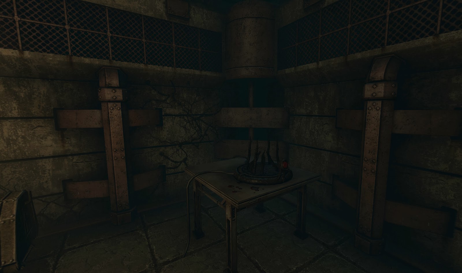
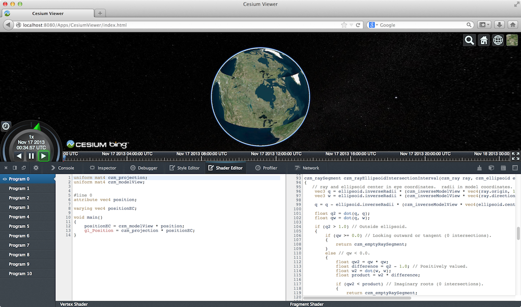
    The Firefox WebGL Shader Editor allows us to view all shader programs in a WebGL app, edit them in real-time, and mouse over them to see what parts of the scene were drawn using them.

    What I like most about it is it actually works. Scenes in our engine usually have 10-50 procedurally-generated shaders that can be up to ~1,000 lines. The shader editor handles this smoothly and automatically updates when new shaders are created.

    skybox

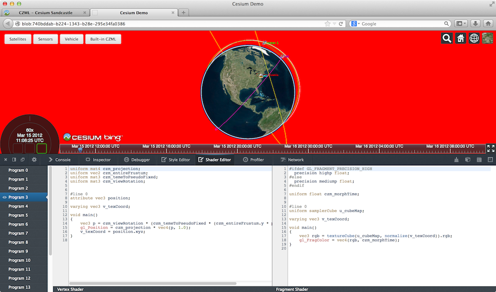
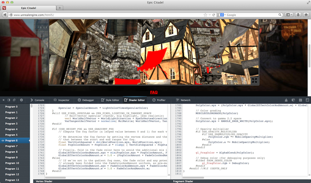
    The skybox shader is shown in the editor and the geometry is highlighted in red. (Click on any image for its full-screen version.)

    I was very impressed to see the shader editor also work on the Epic Citadel demo, which has 249 shaders, some of which are ~2,000 lines.

    citadel

    Live editing is, of course, limited. For example, we can’t add new uniforms and attributes and provide data for them; however, we can add new varying variables to pass data between vertex and fragment shaders.

    Given that the editor needs to recompile after our edits, attribute and uniform locations could change, e.g., if uniforms are optimized out, which would break most apps (unless the app is querying these every frame, which is a terrible performance idea). However, the editor seems to handle remapping under-the-hood since removing uniforms doesn’t break other uniforms.

    Recompiling after typing stops works well even for our large shaders. However, every editor I see like this, including JavaScript ones we’ve built, tends to remove this feature in favor of an explicit run, as the lag can otherwise be painful.

    There are some bugs, such as mousing over some shaders causes artifacts or parts of the scene to go away, which makes editing those shaders impossible.

    artifacts

    Even though this is in a pre-beta version of Firefox, I find it plenty usable. Other than spot testing, I use Chrome for development, but this tool really makes me want to use Firefox, at least for shader debugging.

    We planned to write a tool like this for our engine, but I’m glad the Mozilla folks did it instead since it benefits the entire WebGL community. An engine-specific tool will still be useful for some. For example, this editor uses the shader source provided to WebGL. If a shader is procedurally-generated, an engine-specific editor can present the individual snippets, nodes in a shade tree, etc.

    A few features that would make this editor even better include:

    • Make boldface any code in #ifdef blocks that evaluate to true. This is really useful for ubershaders.
    • Mouse over a pixel and show the shader used. Beyond debugging, this would be a great teaching aid and tool for understanding new apps. I keep pitching the idea of mousing over a pixel and then showing a profile of the fragment shader as a final project to my students, but no one ever bites. Easy, right?
    • An option to see only shaders actually used in a frame, instead of all shaders in the WebGL context, since many shaders can be for culled objects. Taking it a step further, the editor could show only shaders for non-occluded fragments.

    For a full tutorial, see Live editing WebGL shaders with Firefox Developer Tools.

    WebGL Inspector

    The WebGL Inspector was perhaps the first WebGL debugging tool. It hasn’t been updated in a long time, but it is still useful.

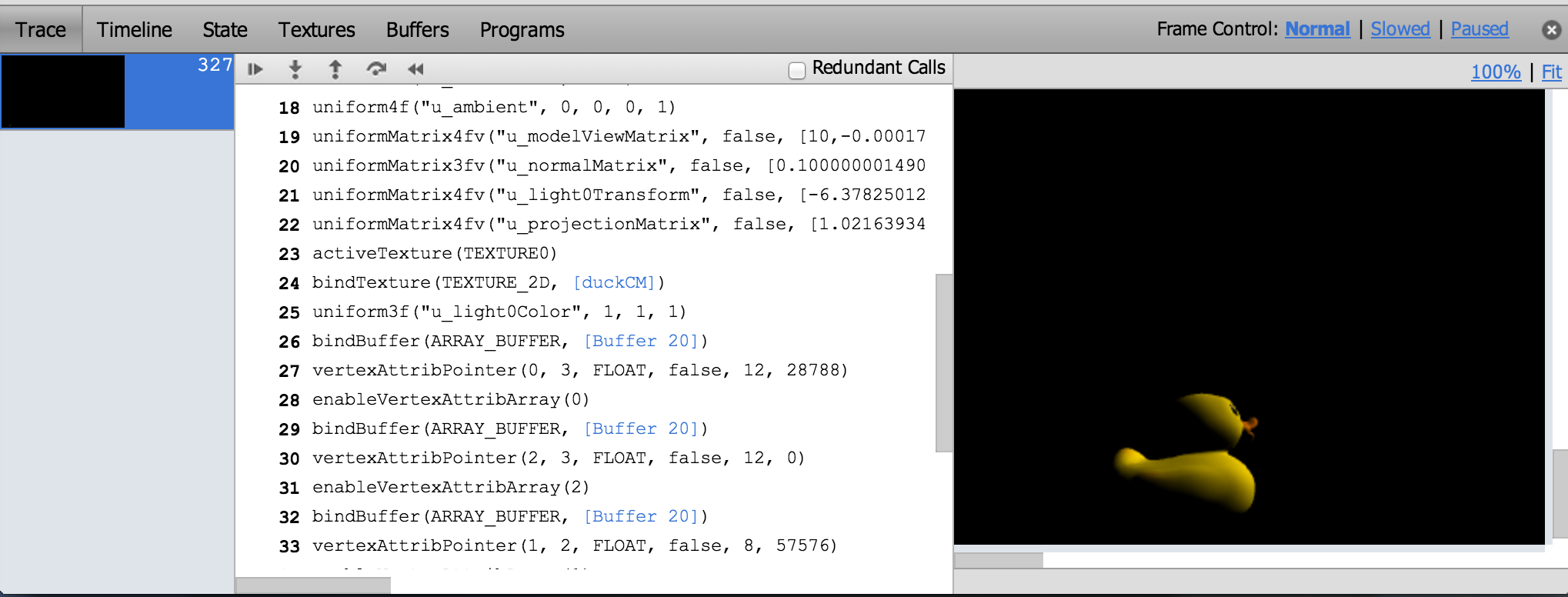
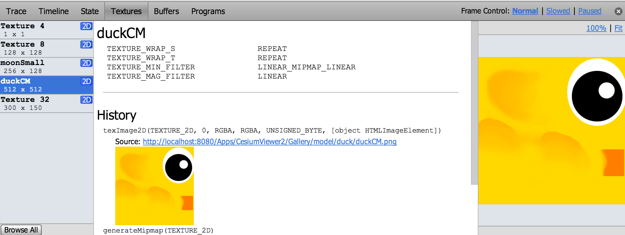
    WebGL Inspector can capture a frame and step through it, building the scene one draw call at a time; view textures, buffers, state, and shaders; etc.

    The trace shows all the WebGL calls for a frame and nicely links to more info for function arguments that are WebGL objects. We can see the contents and filter state of textures, contents of vertex buffers, and shader source and current uniforms.

    ducktrace

    ducktexture

    One of WebGL Inspector’s most useful features is highlighting redundant WebGL calls, which I use often when doing analysis before optimizing.

    redundant

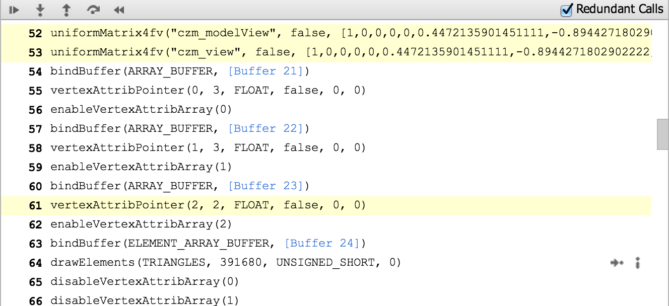
    Like most engines, setting uniforms is a common bottleneck for us and we are guilty of setting some redundant uniforms for now.

    WebGL Inspector may take some patience to get good results. For our engine, the scene either isn’t visible or is pushed to the bottom left. Also, given its age, this tool doesn’t know about extensions such as Vertex Array Objects. So, when we run our engine with WebGL Inspector, we don’t get the full set of extensions supported by the browser.

    The WebGL Inspector page has a full walkthrough of its features.

    Chrome Canvas Inspector

    The Canvas Inspector in Chrome DevTools is like a trimmed-down WebGL Inspector built right into Chrome. It is an experimental feature but available in Chrome stable (Chrome 31). In chrome://flags/, “Enable Developer Tools experiments” needs to be checked and then the inspector needs to be explicitly enabled in the DevTools settings.

    Although it doesn’t have nearly as many features as WebGL Inspector, Canvas Inspector is integrated into the browser and trivial to use once enabled.

    canvasinspector

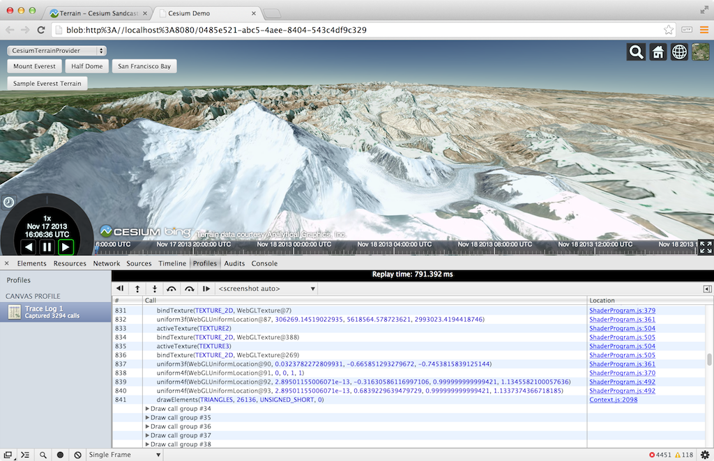
    Draw calls are organized into groups that contain the WebGL state calls and the affected draw call. We can step one draw group or one WebGL call at a time (all WebGL tracing tools can do this). The scene is supposed to be shown one draw call at a time, but we currently need to turn off Vertex Array Objects for it to work with our engine. Canvas Inspector can also capture consecutive frames pretty well.

    The inspector is nicely integrated into the DevTools so, for example, there are links from a WebGL call to the line in the JavaScript file that invoked it. We can also view the state of resources like textures and buffers, but not their contents or history.

    Tools like WebGL Inspector and Canvas Inspector are also useful for code reviews. When we add a new rendering feature, I like to profile and step through the code as part of the review, not just read it. We have found culling bugs when stepping through draw calls and then asking why there are so many that aren’t contributing to any pixels.

    For a full Canvas Inspector tutorial, see Canvas Inspection using Chrome DevTools.

    Google Web Tracing Framework

    The Google Web Tracing Framework (WTF) is a full tracing framework, including support for WebGL similar to WebGL Inspector and Canvas Inspector. It is under active development on github; they addressed an issue I submitted in less than a day! Even without manually instrumenting our code, we can get useful and reliable results.

    Here we’re stepping through a frame one draw call at a time:

    wtf

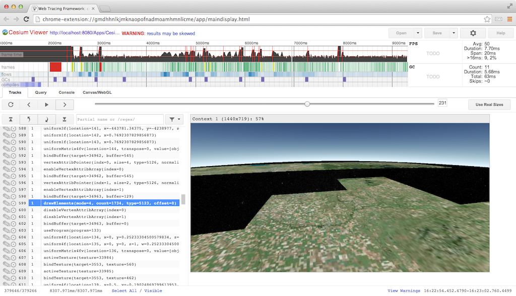
    For WebGL, WTF has similar trace capability as the above inspectors, combined with all its general JavaScript tracing features. The WebGL trace integrates nicely with the tracks view.

    tracks

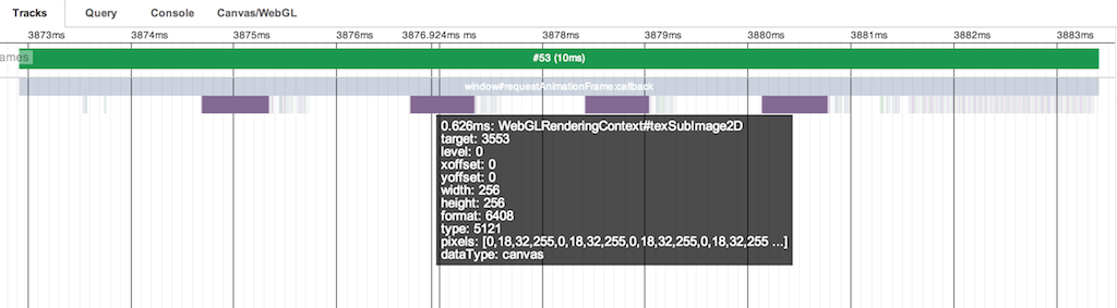
    Above, we see the tracks for frame #53. The four purple blocks are texture uploads using texSubImage2D to load new imagery tiles we received from a web worker. Each call is followed by several WebGL state calls and a drawElements call to reproject the tile on the GPU (see World-Scale Terrain Rendering from the Rendering Massive Virtual Worlds SIGGRAPH 2013 course). The right side of the frame shows all the state and draw calls for the actual scene.

    Depending on how many frames the GPU is behind, a better practice would be to do all the texSubImage2D calls, followed by all the reprojection draw calls, or even move the reprojection draw calls to the end of the frame with the scene draw calls. The idea here is to ensure that the texture upload is complete by the time the reprojection draw call is executed. This trades the latency of completing any one for the throughput of computing many. I have not tried it in this case so I can’t say for certain if the driver lagging behind isn’t already enough time to cover the upload.

    gc

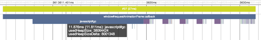
    The tracks view gets really interesting when we examine slow frames highlighted in yellow. Above, the frame takes 27ms! It looks similar to the previous frame with four texture uploads followed by drawing the scene, but it’s easy to see the garbage collector kicked in, taking up almost 12ms.

    linkProgram

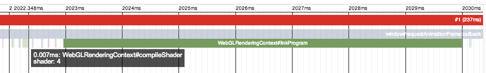
    Above is our first frame, which takes an astounding 237ms because it compiles several shaders. The calls to compileShader are very fast because they don’t block, but the immediate call to linkProgram needs to block, taking ~7ms for the one shown above. A call to getShaderParameter or getShaderInfoLog would also need to block to compile the shader. It is a best practice to wait as long as possible to use a shader object after calling compileShader to take advantage of asynchronous driver implementations. However, testing on my MacBook Pro with an NVIDIA GeForce 650M did not show this. Putting a long delay before linkProgram did not decrease its latency.

    For more details, see the WTF Getting Started page. You may want to clear a few hours.

    More Tools

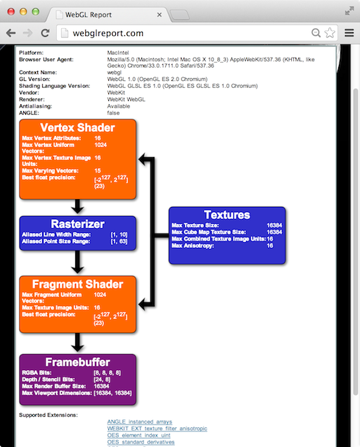
    The WebGL Report is handy for seeing a system’s WebGL capabilities, including extensions, organized by pipeline stage. It’s not quite up-to-date with all the system-dependent values for the most recent extensions, but it’s close. Remember, to access draft extensions in Chrome, we need to explicitly enable them in the browser now. For enabling draft extensions in Firefox you need to go to “about:config” and set the “webgl.enable-draft-extensions” preference to true.

    webglreport

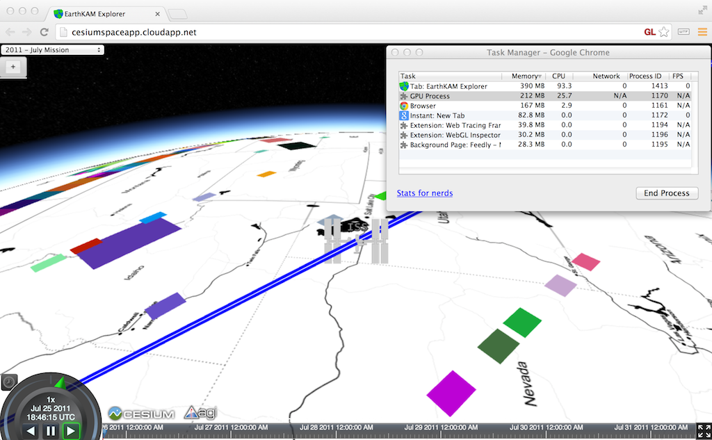
    The simple Chrome Task Manager (in the Window menu) is useful for quick and dirty memory usage. Make sure to consider both your app’s process and the GPU process.

    taskmanager

    Although I have not used it, webgl-debug.js wraps WebGL calls to include calls to getError. This is OK for now, but we really need KHR_debug in WebGL to get the debugging API desktop OpenGL has had for a few years. See ARB_debug_output: A Helping Hand for Desperate Developers in OpenGL Insights.

    There are also WebGL extensions that provide debugging info to privileged clients (run Chrome with –enable-privileged-webgl-extensions). WEBGL_debug_renderer_info provides VENDOR and RENDERER strings. WEBGL_debug_shaders provides a shader’s source after it was translated to the host platform’s native language. This is most useful on Windows where ANGLE converts GLSL to HLSL. Also see The ANGLE Project: Implementing OpenGL ES 2.0 on Direct3D in OpenGL Insights.

    The Future

    The features expected in WebGL 2.0, such as multiple render targets and uniform buffers, will bring us closer to the feature-set OpenGL developers have enjoyed for years. However, API features alone are not enough; we need an ecosystem of tools to create an attractive platform.

    Building WebGL tools, such as the Firefox Shader Editor and Chrome Canvas Inspector, directly into the browser developer tools is the right direction. It makes the barrier to entry low, especially for projects with limited time or developers. It helps more developers use the tools and encourages using them more often, for the same reason that unit tests that run in the blink of an eye are then used frequently.

    The current segmentation of Google’s tools may appear confusing but I think it shows the evolution. WebGL Inspector was first out of the gate and proved very useful. Because of this, the next generation version is being built into Chrome Canvas Inspector for easy access and into the WTF for apps that need careful, precise profiling. For me, WTF is the tool of choice.

    We still lack a tool for setting breakpoints and watch variables in shaders. We don’t have what NVIDIA Nsight is to CUDA, or what AMD CodeXL is to OpenCL. I doubt that browser vendors alone can build these tools. Instead, I’d like to see hardware vendors provide back-end support for a common front-end debugger built into the browser.

    21 Oct 07:50

    Link collection of temporal coherence methods for realtime rendering

    by hanecci

    Reference

    Temporal coherence methods for realtime rendering

    21 Oct 07:50

    Link collection of fast GPU filtering techniques for averaging pixel values

    by hanecci

    Reference

    Techniques

    21 Oct 07:50

    Link collection of SSAO techniques

    by hanecci

    Reference

    SSAO techniques

    • (a) CryEngine 2 AO

    f:id:hanecci:20131021024119j:image:w360

    • (b) StarCraft2 AO

    f:id:hanecci:20131021024133j:image:w360

    • (c) Horizontal Ambient Occlusion (HBAO)

    f:id:hanecci:20131021024146j:image:w360

    • (d) Volumetric Obscurance

    f:id:hanecci:20131021024313j:image:w360

    • (e) Alchemy AO

    f:id:hanecci:20131021024517j:image:w360

      • (In Japanese) 概略
        • スクリーンスペースで円盤上をランダムサンプリングして, Horizon Angle に相当する dot(n, v)の平均値を求めます.
    • (f) Unreal Engine 4 AO

    f:id:hanecci:20131021024704j:image:w360

    21 Oct 07:44

    Porting from DirectX11 to OpenGL 4.2: API mapping

    by Anteru

    Welcome to my Direct3D to OpenGL mapping cheat-sheet, which will hopefully help you to get started with adding support for OpenGL to your renderer. The hardest part for me during porting is to find out which OpenGL API corresponds to a specific Direct3D API call, and here is a write-down of what I found out & implemented in my rendering engine. If you find a mistake, please drop me a line so I can fix it!

    Device creation & rendering contexts

    In OpenGL, I go through the usual hoops: That is, I create an invisible window, query the extension functions on that, and then finally go on to create an OpenGL context that suits me. For extensions, I use glLoadGen which is by far the easiest and safest way to load OpenGL extensions I have found.

    I also follow the Direct3D split of a device and a device context. The device handles all resource creation, and the device context handles all state changes. As using multiple device contexts is not beneficial for performance, my devices only expose the “immediate” context. That is, in OpenGL, a context is just use to bundle the state changing functions, while in Direct3D, it wraps the immediate device context.

    Object creation

    In OpenGL, everything is an unsigned integer. I wrap every object type into a class, just like in Direct3D.

    Vertex and index buffers

    Work similar to Direct3D. Create a new buffer using glGenBuffers, bind it to either vertex storage (GL_ARRAY_BUFFER) or to index storage (GL_ELEMENT_ARRAY_BUFFER) and populate it using glBufferData.

    Buffer mapping

    Works basically the same in OpenGL as in Direct3D, just make sure to use glMapBufferRange and not glMapBuffer, which gives you better control over how the data is mapped, and makes it easy to guarantee that no synchronization happens. With glMapBufferRange, you can mimic the Direct3D behaviour perfectly and with the same performance.

    Rasterizer state

    This maps directly to OpenGL; but it’s split across several functions: glPolygonMode, glEnable/Disable for things like culling, glCullFace, etc.

    Depth/Stencil state

    Similar to the rasterizer state, you need to use glEnable/Disable to set things like the depth test, and then glDepthMask, glDepthFunc, etc.

    Blend state

    And another state which is split across several functions. Here we’re talking about glEnable/Disable for blending in general, then glBlendEquationi to set the blend equations, glColorMaski, glBlendFunci and glBlendColor. The functions with the i suffix allow you to set the blending equations for each “blend unit” just as in Direct3D.

    Vertex layouts

    I require a similar approach to Direct3D here. First of all, you can create one vertex layout per vertex shader program. This allows me to query the location of all attributes using glGetAttribLocation and store them for the actual binding later.

    At binding time, I bind the vertex buffer first, and then set the layout for it. I call glVertexAttribPointer (or glVertexAttribIPointer, if it is an integer type) followed by glEnableVertexAttribArray and glVertexAttribDivisor to handle per-instance data. Setting the layout after the vertex buffer is bound allows me to handle draw-call specific strides as well. For example, I sometimes render with a stride that is a multiple of the vertex size to skip data, which has to be specified using glVertexAttribPointer (unlike in Direct3D, where this is a part of the actual draw call.)

    The better solution here is to use ARB_vertex_attrib_binding, which would map directly to a vertex layout in Direct3D parlance and which does not require lots of function calls per buffer. I’m not sure how this interacts with custom vertex strides, though.

    Draw calls

    That’s pretty simple once the layouts are bound, as you have to handle the stride setting there. Once this is resolved, just pick the function which maps to the Direct3D equivalent:

    Textures & samplers

    First, storing texture data. Currently I use glTexImage2D and glCompressedTexImage2D for each mip-map individually. The only problem here is to handle the internal format, format and type for OpenGL — I store them along with the texture, as they are all needed at some point. Using glTexImage2D is however not the best way to define texture storage. These APIs allow you to resize a texture later on, which is something Direct3D doesn’t, and the same behaviour can be obtained in OpenGL using the glTexStorage2D​ function. This allocates and fixes the texture storage, and only allows you to upload new data.

    Uploading and downloading data is the next part. For a simple update (where I use UpdateSubresource in Direct3D), I simply replace all image data using glTexSubImage2D. For mapping I allocate a temporary buffer and on unmap, I call glTexImage2D to replace the storage. Not sure if this is the recommended solution, but it works and allows for the same host code as Direct3D.

    Binding textures and samplers is a more involved topic that I have previously blogged about in more detail. It boils down to statically assigning texture slots to shaders, and manually binding them to samplers and textures. I simply chose to add a new #pragma to the shader source code which I handle in my shader preprocessor to figure out which texture to bind to which slot, and which sampler to bind. On the Direct3D side, this requires me to use numbered samplers, to allow the host & shader code to be as similar as possible.

    Texture buffers work just like normal buffers in OpenGL, but you have to associate a texture with your texture buffer. That is, you create a normal buffer first using glBindBuffer and GL_TEXTURE_BUFFER as the target, and with this buffer bound, you bind a texture to it and populate it using glTexBuffer.

    Constant buffers

    This maps to uniform buffers in OpenGL. One major difference is where global variables end up, in Direct3D, they are put into a special constant buffer called $Global, in OpenGL they have to be set directly. I added special-case handling for global variables to shader programs; in OpenGL, they set the variables directly and in Direct3D globals are set through a “hidden” constant buffer which is only uploaded when the shader is actually bound.

    The nice thing about OpenGL is that it gives you binding of sub-parts of a buffer for free. Instead of using glBindBufferBase to bind the complete constant buffer, you simply use glBindBufferRange, no need to fiddle around with difference device context versions as in Direct3D.

    Shaders

    I use the separate shader programs extension to handle this. Basically, I have a pipeline bound with all stages set and when a shader program is bound, I use glUseProgramStages to set it to its correct slot. The only minor difference here is that I don’t use  glCreateShaderProgram, but instead, I do the steps manually. This allows me to access the set the binary shader program hint (GL_PROGRAM_BINARY_RETRIEVABLE_HINT), which you cannot obtain otherwise. Oh I grab the shader program log manually as well, as there is no way from client code to append the shader info log to the program info log.

    For shader reflection, the API is very similar. First, you query how many constant buffers and uniforms a program has using glGetProgramiv. Then, you can use glGetActiveUniform to query a global variable and glGetActiveUniformBlockiv, glGetActiveUniformBlockName to query everything about a buffer.

    Unordered access views

    These are called image load/store in OpenGL. You can take a normal texture and bind it to an image unit using glBindImageTexture. In the shader, you have a new data type called image2D or imageBuffer, which is the equivalent to an unordered access view.

    Acknowledgements

    That’s it. What I found super-helpful during porting was the OpenGL wiki and the 8th edition of the OpenGL programming guide. Moreover, thanks to the following people (in no particular order): Johan Andersson of DICE fame who knows the performance of every Direct3D API call, Aras Pranckevičius, graphics guru at Unity, Christophe Riccio, who has used every OpenGL API call, and Graham Sellers, who has probably implemented every OpenGL API call.

    21 Oct 07:43

    Link collection of Voxel based Global Illumination

    by hanecci

    Cyril Crassin

    Others

    21 Oct 07:43

    Link collection of tile based deferred shading

    by hanecci