Want to go off-road? This jam-packed tutorial offers C++ code snippets for simulating water, mud, and different lighting conditions in a natural driving environment. ...
Personally I think that Plants vs. Zombies 2 (PvZ2) is a great game. The game has kept all the good from the first episode and spiced it up with new content as well as features like map and gesture operated powerups. The biggest change of the sequel though is that it wen from paid to free. And as you know, this blog is all about game mechanic.
In hindsight it seems that dropping the
This is short guide how to create parallax effect using accelerometer on mobile platforms. Some code is related to Android, but all concept is applicable to iOS, etc.
What is parallax effect? There are some more complex definitions but i would define as simple as the following – you move your phone/device in space and some objects inside your application are shifting accordingly to compensate this movement. This allows to create some strong feeling of 3d interface as well as nice interaction effect.
As good example you can check out my live wallpaper (link on market), which is using this effect while rendering particle system of moving objects. More information about this application can be found here.
To create parallax effect we need to grab data from accelerometer sensor (as i found out gyroscope is not present at majority of phones while accelerometer gives enough of data to be happy with it), convert sensor data to relative rotation angles and shift some parts of application interface accordingly. 3 steps:
1. Get data from accelerometer
You can read here about usage of motion sensor inside android sdk. (I provide some code here for Android just as sample – approach should be same for iOS)
As any measurement system sensor has noise and you can filter input data using one of signal filters such as low-pass filter – but the most simple way to do it is the following:
Filtering constant can depend on sensor frequency, but the tricky part is that you cant get frequency as some property and have to measure it directly. Speed can vary from device to device considerably from 7 Hz to 100Hz (source). I found that under 25Hz effect becomes less entertaining and should be disabled, unless you make prediction approximation and perform heavy smooth on input data.
2. Convert accelerometer data to rotation angles
Second task is to get device orientation angles from gravity vector. I use the following formula to get roll and pitch values (desired angles):
Note that if device orientation was changed to landscape mode you need to swap roll and pitch values. Also atan2 function can produce 2pi jumps and we can just ignore such events. We dont need absolute angle values – only difference with previous device state (dgX, dgY):
// normalize gravity vector at first
double gSum = sqrt(gX*gX + gY*gY + gZ*gZ);
if (gSum != 0)
{
gX /= gSum;
gY /= gSum;
gZ /= gSum;
}
if (gZ != 0)
roll = atan2(gX, gZ) * 180/M_PI;
pitch = sqrt(gX*gX + gZ*gZ);
if (pitch != 0)
pitch = atan2(gY, pitch) * 180/M_PI;
dgX = (roll – lastGravity[0]);
dgY = (pitch – lastGravity[1]);
// if device orientation is close to vertical – rotation around x is almost undefined – skip!
if (gY > 0.99) dgX = 0;
// if rotation was too intensive – more than 180 degrees – skip it
if (dgX > 180) dgX = 0;
if (dgX < -180) dgX = 0;
if (dgY > 180) dgY = 0;
if (dgY < -180) dgY = 0;
if (!screen->isPortrait())
{
// Its landscape mode – swap dgX and dgY
double temp = dgY;
dgY = dgX;
dgX = temp;
}
lastGravity[0] = roll;
lastGravity[1] = pitch;
So we have angle shifts inside dgX, dgY variables and can proceed to final step.
3. Perform interface shift
And as final step we need to shift some elements inside application to compensate device rotation. In my case that was particle system – for each particle we perform x/y shift proportionally current particle depth (if it’s 3d environment you can also perform some rotations to make ideal compensation) .
// Parallax effect – if gravity vector was changed we shift particles
if ((dgX != 0) || (dgY != 0))
{
p->x += dgX * (1. + 10. * p->z);
p->y -= dgY * (1. + 10. * p->z);
}
Only practice can help to find optimal coefficients for such shifts which are different for every application. You can shift background details or foreground decorations.
Couple of small details: sensor events and rendering should be done in separate threads. And when device goes to sleep you should unregister sensor listener (and so dont waste battery).
UPDATE: This post sucks; it has some useful bits about setting up a breakpoint in the Xcode debugger – but apart from that: I recommend skipping it and going straight to Part 4b instead, which explains things much better.
This is Part 4, and explains how to debug in OpenGL, as well as improving some of the reusable code we’ve been using (Part 1 has an index of all the parts, Part 3 covered Geometry).
Last time, I said we’d go straight to Textures – but I realised we need a quick TIME OUT! to cover some code-cleanup, and explain in detail some bits I glossed-over previously. This post will be a short one, I promise – but it’s the kind of stuff you’ll probably want to bookmark and come back to later, whenever you get stuck on other parts of your OpenGL code.
NB: if you’re reading this on AltDevBlog, the code-formatter is currently broken on the server. Until the ADB server is fixed, I recommend reading this (identical) post over at T-Machine.org, where the code-formatting is much better.
Cleanup: VAOs, VBOs, and Draw calls
In the previous part, I deliberately avoided going into detail on VAO (Vertex Array Objects) vs. VBO (Vertex Buffer Objects) – it’s a confusing topic, and (as I demonstrated) you only need 5 lines of code in total to use them correctly! Most of the tutorials I’ve read on GL ES 2 were simply … wrong … when it came to using VAO/VBO. Fortunately, I had enough experience of Desktop GL to skip around that – and I get the impression a lot of GL programmers do the same.
Let’s get this clear, and correct…
To recap, I said last time:
A VertexBufferObject:
…is a plain BufferObject that we’ve filled with raw data for describing Vertices (i.e.: for each Vertex, this buffer has values of one or more ‘attribute’s)
Each 3D object will need one or more VBO’s.
When we do a Draw call, before drawing … we’ll have to “select” the set of VBO’s for the object we want to draw.
A VertexArrayObject:
…is a GPU-side thing (or “object”) that holds the state for an array-of-vertices
It records info on how to “interpret” the data we uploaded (in our VBO’s) so that it knows, for each vertex, which bits/bytes/offset in the data correspond to the attribute value (in our Shaders) for that vertex
Vertex Buffer Objects: identical to any other BufferObject
It’s important to understand that a VBO is a BO, and there’s nothing special or magical about it: everything you can do with a VBO, you can do with any BO. It gets given a different name simply because – at a few key points – you need to tell OpenGL “interpret the data inside this BO as if it’s vertex-attributes … rather than (something else)”. In practice, all that means is that:
If you take any BO (BufferObject), every method call in OpenGL will require a “type” parameter. Whenever you pass-in the type “GL_ARRAY_BUFFER”, you have told OpenGL to use that BO as a VBO. That’s all that VBO means.
…the hardware may also (perhaps; it’s up to the manufacturers) do some behind-the-scenes optimization, because you’ve hinted that a particular BO is a VBO – but it’s not required.
Vertex Buffer Objects: why plural?
In our previous example, we had only one VBO. It contained only one kind of vertex-attribute (the “position” attribute). We used it in exactly one draw call, for only one 3D object.
A BufferObject is simply a big array stored on the GPU, so that the GPU doesn’t have to keep asking for the data from system-RAM. RAM -> GPU transfer speeds are 10x slower than GPU-local-RAM (known as VRAM) -> GPU upload speeds.
So, as soon as you have any BufferObjects, your GPU has to start doing memory-management on them. It has its own on-board caches (just like a CPU), and it has its own invisible system that intelligently pre-fetches data from your BufferObjects (just like a CPU does). This then begs the question:
What’s the efficient way to use BufferObjects, so that the GPU has to do the least amount of shuffling memory around, and can maximize the benefit of its on-board caches?
The short answer is:
Create one single VBO for your entire app, upload all your data (geometry, shader-program variables, everything), and write your shaders and draw-calls to use whichever subsets of that VBO apply to them. Never change any data.
OpenGL ES 2 doesn’t fully support that usage: some of the features necessary to put “everything” into one VBO are missing. Also: if you start to get low on spare memory, if you only have one VBO, you’re screwed. You can’t “unload a bit of it to make more room” – a VBO is, by definition, all-or-nothing.
How do Draw calls relate to VBO’s?
This is very important. When you make a Draw call, you use glVertexAttribPointer to tell OpenGL:
“use the data in BufferObject (X), interpreted according to rule (Y), to provide a value of this attribute for EACH vertex in the object”
…a Draw call has to take the values of a given attribute all at once from a single VBO. Incidentally, this is partly why I made the very first blog post teach you about Draw calls – they are the natural atomic unit in OpenGL, and life is much easier if you build your source-code around that assumption.
So, bearing in mind the previous point about wanting to load/unload VBOs at different times … with GL ES 2, you divide up your VBO’s in two key ways, and stick to one key rule:
Any data that might need to be changed while the program is running … gets its own VBO
Any data that is needed for a specific draw-call, but not others … gets its own VBO
RULE: The smallest chunk of data that goes in a VBO is “the attribute values for one attribute … for every vertex in an object”
…you can have the values for more than one Attribute inside a single VBO – but it has to cover all the vertices, for each Attribute it contains.
A simple VBO class (only allows one Attribute per VBO)
For highest performance, you normally want to put multiple Attributes into a single VBO … but there are many occasions where you’ll only use 1:1, so let’s start there.
The first two properties are fairly obvious. We have our standard “glName” (everything has one), and we have a glBufferType, which is set to GL_ARRAY_BUFFER whenever we want the BO to become a VBO.
To understand the next part, we need to revisit the 3 quick-n-dirty lines we used in the previous article:
…the first two lines are simply creating a BO/VBO, and storing its name. And we’ll be able to automatically supply the “GL_ARRAY_BUFFER” argument from now on, of course. Looking at that last line, the second-to-last argument is “the array of data we created on the CPU, and want to upload to the GPU” … but what’s the second argument? A hardcoded “3 * (something)”? Ouch – very bad practice, hardcoding a digit with no explanation. Bad coder!
glBufferData requires, as its second argument:
(2nd argument): The total amount of RAM I need to allocate on the GPU … to store this array you’re about to upload
In our case, we were uploading 3 vertices (one for each corner of a triangle), and each vertex was defined using GLKVector3. The C function “sizeof” is a very useful one that measures “how many bytes does a particular type use-up when in memory?”.
So, for our GLK2BufferObject class to automatically run glBufferData calls in future, we need to know how much RAM each attribute-value occupies:
…and if you read the OpenGL method-docs, you’d see that the 2nd argument there is also called “size” – but we used a completely different number!
And, finally, when we issue the Draw call, we use the number 3 again, for a 3rd kind of ‘size’:
(from previous blog post)
glDrawArrays( GL_TRIANGLES, 0, 3); // this 3 is NOT THE SAME AS PREVIOUS 3 !
WTF? Three definitions of “size” – O, RLY?
Ya, RLY.
glBufferData: measures size in “number of bytes needed to store one Attribute-value”
glVertexAttribPointer: measures size in “number of floats required to store one Attribute-value”
glDrawArrays: measures size in “number of vertices to draw, out of the ones in the VBO” (you can draw fewer than all of them)
For the final one – glDrawArrays – we’ll store that data (how many vertices to “draw”) in the GLK2DrawCall class itself. But we’ll need to store the info for glVertexAttribPointer inside each VBO:
Now we can implement GLK2BufferObject.m, and remove the hard-coded numbers from our previous source code:
GLK2BufferObject.m:
[objc]
…
-(void) upload:(void *) dataArray numItems:(int) count usageHint:(GLenum) usage
{
NSAssert(self.bytesPerItem > 0 , @”Can’t call this method until you’ve configured a data-format for the buffer by setting self.bytesPerItem”);
NSAssert(self.glBufferType > 0 , @”Can’t call this method until you’ve configured a GL type (‘purpose’) for the buffer by setting self.glBufferType”);
The only special item here is “usage”. Previously, I used the value “GL_DYNAMIC_DRAW”, which doesn’t do anything specific, but warns OpenGL that we might choose to re-upload the contents of this buffer at some point in the future. More correctly, you have a bunch of different options for this “hint” – if you look at the full source on GitHub, you’ll see a convenience method and two typedef’s that handle this for you, and explain the different options.
Source for: GLK2BufferObject.h and GLK2BufferObject.m
VertexArrayObject: stores the metadata for “which VBOs are you using, what kind of data is inside them, how can a ShaderProgram read and interpret that data, etc”
We’ll start with a new class with the (by now: obvious) properties and methods:
/** Delegates to the other method, defaults to using “GL_STATIC_DRAW” as the BufferObject update frequency */
-(GLK2BufferObject*) addVBOForAttribute:(GLK2Attribute*) targetAttribute filledWithData:(void*) data bytesPerArrayElement:(GLsizeiptr) bytesPerDataItem arrayLength:(int) numDataItems;
/** Fully configurable creation of VBO + upload of data into that VBO */
-(GLK2BufferObject*) addVBOForAttribute:(GLK2Attribute*) targetAttribute filledWithData:(void*) data bytesPerArrayElement:(GLsizeiptr) bytesPerDataItem arrayLength:(int) numDataItems updateFrequency:(GLK2BufferObjectFrequency) freq;
@end
[/objc]
The method at the end is where we move the very last bit of code from the previous blog post – the stuff about glVertexAttribPointer. We also combine it with automatically creating the necessary GLK2BufferObject, and calling the “upload:numItems:usageHint” method:
GLK2VertexArrayObject.m:
[objc]
…
-(GLK2BufferObject*) addVBOForAttribute:(GLK2Attribute*) targetAttribute filledWithData:(void*) data bytesPerArrayElement:(GLsizeiptr) bytesPerDataItem arrayLength:(int) numDataItems updateFrequency:(GLK2BufferObjectFrequency) freq
{
/** Create a VBO on the GPU, to store data */
GLK2BufferObject* newVBO = [GLK2BufferObject vertexBufferObject];
newVBO.bytesPerItem = bytesPerDataItem;
[self.VBOs addObject:newVBO]; // so we can auto-release it when this class deallocs
/** Send the vertex data to the new VBO */
[newVBO upload:data numItems:numDataItems usageHint:[newVBO getUsageEnumValueFromFrequency:freq nature:GLK2BufferObjectNatureDraw]];
/** Configure the VAO (state) */
glBindVertexArrayOES( self.glName );
Anyone with sharp eyes will notice that I uploaded “vector3″ (data in the form: x,y,z) to an attribute of type “vector4″ (data in the form: x,y,z,w). And nothing went wrong. Huh?
The secret here is two fold:
OpenGL’s shader-language is forgiving and smart; if you give it a vec3 where it needs a vec4, it will up-convert automatically
We told all of OpenGL “outside” the shader-program: this buffer contains Vector3′s! Each one has 3 floats! Note: That’s THREE! Not FOUR!
…otherwise, I’d have had to define our triangle using 4 co-ordinates – and what the heck is the correct value of w anyway? Better not to even go there (for now). All of this “just works” thanks to the code we’ve written above, in this post. We explicitly tell OpenGL how to interpret the contents of a BufferObject even though the data may not be in the format the shader is expecting – and then OpenGL handles the rest for us automagically.
Errors – ARGH!
We’re about to deal with “textures” in OpenGL – but we have to cover something critical first.
In previous parts, each small feature has required only a few lines of code to achieve even the most complex outcomes … apart from “compiling and linking Shaders”, which used many lines of boilerplate code.
Texture-mapping is different; this is where it gets tough. Small typos will kill you – you’ll get “nothing happened”, and debugging will be near to impossible. It’s time to learn how to debug OpenGL apps.
OpenGL debugging: the glGetError() loop
There are three ways that API’s / libraries return errors:
(very old, C-only, APIs): An integer return code from every method, that is “0″ for success, and “any other number” for failure. Each different number flags a different cause / kind of error
(old, outdated APIs): An “error” pointer that you pass in, and MAY be filled-in with an error if things go wrong. Apple does a variant of this with most of their APIs, although they don’t need to any more (it used to be “required”, but they fixed the problems that forced that, and it’s now optional. Exceptions work fine)
(modern programming languages and APIs): If something goes wrong, an Exception is thrown (modern programming languages do some Clever Tricks that make this exactly as fast as the old methods, but much less error-prone to write code with)
Then there’s another way. An insane, bizarre, way … from back when computers were so new, even the C-style approach hadn’t become “standard” yet. This … is what OpenGL uses:
Every method always succeeds, even when it fails
If it fails, a “global list of errors” is created, and the error added to the end
No error is reported – no warnings, no messages, no console-logs … nothing
If other methods fail, they append to the list of errors
At any time, you can “read” the oldest error, and remove it from the list
In fairness, there was good reason behind it. They were trying to make an error-reporting system that was so high-performance it had zero impact on the runtime. They were also trying to make it work over the network (early OpenGL hardware was so special/expensive, it wasn’t even in the same machine you ran your app on – it lived on a mainframe / supercomputer / whatever in a different room in your office).
It’s important to realise that the errors are on a list – if you only call “if( isError )” you’ll only check the first item on the list. By the time you check for errors, there may be more-than-one error stacked up. So, in OpenGL, we do our error checking in a while-loop: “while( thereIsAnotherError ) … getError … handleError”.
UPDATE: ignore the rest, use this (Xcode5)
Xcode5 now does 95% of the work for you, in 3 clicks – this is awesome.
Select your Breakpoints tab, hit the (hard to find) plus button at bottom left, and select “OpenGL ES Error”:
This is a magic breakpoint where OpenGL will catch EVERY GL error as soon as it happens and pause in the debugger for you. You should have this permanently enabled while developing!
(if you’re not familiar with Xcode’s catch-all breakpoints, the other one that most devs have always-on is “Exception Breakpoint”, which makes the debugger pause whenever it hits an Exception, and you can see the exact state of your program at the moment the Exception was created. It’s not 100% perfect – some 3rd party libraries (e.g. TestFlight, IIRC) create temporary Exceptions pre-emptively, and get annoying quickly. But it’s pretty good)
What follows is generic code (not dependent on IDE version). I’ll leave it here as an FYI – and in case you ever need to reproduce this logging at runtime, without the debugger (e.g. for remote upload of crash logs to TestFlight or Hockey). But for simple cases: use the Xcode5 feature instead
Using glGetError()
Technically, OpenGL requires you to alternate EVERY SINGLE METHOD CALL with a separate call to “glGetError()”, to check if the previous call had any errors.
If you do NOT do this, OpenGL will DELETE THE INFORMATION about what caused the error.
Since OpenGL ERRORS ARE 100% CONTEXT-SENSITIVE … deleting that info also MAKES THE ERROR TEXT MEANINGLESS.
Painful? Yep. Sorry.
To make it slightly less painful, OpenGL’s “getError()” function also “removes that error from the start of the list” automatically. So you only use one call to achieve both “get-the-current-error”, and “move-to-the-next-one”.
Here’s the source code you have to implement. After every OpenGL call (any method beginning with the letters “gl”):
[objc]
GLenum glErrorLast;
while( (glErrorLast = glGetError()) != GL_NO_ERROR ) // GL spec says you must do this in a WHILE loop
{
NSLog(@”GL Error: %i”, glErrorCapture );
}
[/objc]
This (obviously) makes your source code absurdly complex, completely unreadable, and almost impossible to maintain. In practice, most people do this:
Create a global function that handles all the error checking, and import it to every GL class in your app
Call this function:
Once at the start of each “frame” (remember: frames are arbitrary in OpenGL, up to you to define them)
Once at the start AND end of each “re-usable method” you write yourself – e.g. a “setupOpenGL” method, or a custom Texture-Loader
…
When something breaks, start inserting calls to this function BACKWARDS from the point of first failure, until you find the line of code that actually errored. You have to re-compile / build / test after each insertion. Oh, the pain!
From this post onwards, I will be inserting calls to this function in my sample code, and I won’t mention it further
Standard code for the global error checker
The basic implementation was given above … but we can do a lot better than that. And … since OpenGL debugging is so painful … we really need to do better than that!
We’ll start by converting it into a C-function that can trivially be called from any class OR C code:
[objc]
void gl2CheckAndClearAllErrors()
{
GLenum glErrorLast;
while( (glErrorLast = glGetError()) != GL_NO_ERROR ) // GL spec says you must do this in a WHILE loop
{
NSLog(@”GL Error: %i”, glErrorCapture );
}
}
[/objc]
Improvement 1: Print-out the GL_* error type
OpenGL only allows 6 legal “error types”. All gl method calls have to re-use the 6 types, and they aren’t allowed sub-types, aren’t allowed parameters, aren’t allowed “error messages” to go with them. This is crazy, but true.
First improvement: include the error type in the output.
[objc]
…
while( (glErrorLast = glGetError()) != GL_NO_ERROR ) // GL spec says you must do this in a WHILE loop
{
/** OpenGL spec defines only 6 legal errors, that HAVE to be re-used by all gl method calls. OH THE PAIN! */
NSDictionary* glErrorNames = @{ @(GL_INVALID_ENUM) : @”GL_INVALID_ENUM”, @(GL_INVALID_VALUE) : @”GL_INVALID_VALUE”, @(GL_INVALID_OPERATION) : @”GL_INVALID_OPERATION”, @(GL_STACK_OVERFLOW) : @”GL_STACK_OVERFLOW”, @(GL_STACK_UNDERFLOW) : @”GL_STACK_UNDERFLOW”, @(GL_OUT_OF_MEMORY) : @”GL_OUT_OF_MEMORY” };
Improvement 3: automatically breakpoint / stop the debugger
You know about NSAssert / CAssert, right? If not … go read about it. It’s a clever way to do Unit-Testing style checks inside your live application code, with very little effort – and it automatically gets compiled-out when you ship your app.
We can add an “always-fails (i.e. triggers)” Assertion whenever there’s an error. If you configure Xcode to “always breakpoint on Assertions” (should be the default), Xcode will automatically pause whenever you detect an OpenGL error:
UPDATE:As Chris Ross pointed out, I made a stupid mistake here. To use the __FILE__ etc macros, the way they work (auto-referencing actual lines in source code) you need to make the call itself into a macro, so the compiler re-embeds them in source each time you use them. Modifying code below
NSCAssert( FALSE, @”OpenGL Error; you need to investigate this!” ); // can’t use NSAssert, because we’re inside a C function
}
[/objc]
… see how we create a macro that looks like the function, but expands into the function we need it to be.
Improvement 4: make it vanish from live App-Store builds
By default, Xcode defines a special value for all Debug (i.e. development) builds that is removed for App Store builds.
Let’s wrap our code in an “#if” check that uses this. That way, when we ship our final build to App Store, it will compile-out all the gl error detection. The errors at that point do us no good anyway – users won’t be running the app in a debugger, and the errors in OpenGL are context-sensitive, so error reports from users will do us very little good.
(unless you’re using a remote logging setup, e.g. Testflight/HockeyApp/etc … but in that case, you’ll know what to do instead)
I've just pushed a branch to my fd.o
tree
that brings back the standalone compiler. I've also made some small
enhancements to it. Why? Thanks for asking.
One thing that game developers frequently complain about (and they're
damn right!) is the massive amount of variability among GLSL
compilers. Compiler A accepts a shader, but compiler B generates
errors. Then the real fun begins... which compiler is right? Dig
through the spec, report bugs to the vendors, wait for the vendors to
finger point... it's pretty dire.
Mesa compiler has a reputation of sticking to the letter of the spec.
This has caused some ruffled feathers with game developers and with
some folks in the Mesa community. In cases where our behavior
disagrees with all other shipping implementations, I have submitted
numerous spec bugs. If nobody does what the spec says, you change the
spec.
This isn't to say our conformance is perfect or that we don't have any
bugs. Reality is quite the contrary. However, we are really picky
about stuff that other people aren't quite so picky about. When we
find deviations from the behavior of other implementations, one way or
another, we sort it out.
Sometimes that means changing our behavior (and adding piglit tests).
Sometimes that means changing our behavior (and getting the spec changed).
Sometimes that means implementing a work-around for specific apps
(that is only enabled for those apps!).
Sometimes that means not changing anything (and taking a hard line that
someone else needs to fix their code).
The combination of our ability to build our compiler on many common
platforms and our spec pedanticism puts Mesa in a fairly interesting
position. It means that developers could use our compiler, without
the baggage of the rest of a driver, as the thrid-party to settle
disputes. It can be the "if it compiles on here, it had better
compile anywhere" oracle.
Even if it fails at that, we emit a lot of warnings. Sometimes we emit too
many warnings. A
standalone compiler gives a good start for "lint" for GLSL.
There are already a couple places that we give portability warnings (things we
accept that some compilers are known to incorrectly reject), so there's
already some value there.
Tiantian Liu, Adam Bargteil, James F. O’Brien, Ladislav Kavan
We describe a scheme for time integration of mass-spring systems that makes use of a solver based on block coordinate descent. This scheme provides a fast solution for classical linear (Hookean) springs. We express the widely used implicit Euler method as an energy minimization problem and introduce spring directions as auxiliary unknown variables. The system is globally linear in the node positions, and the non-linear terms involving the directions are strictly local. Because the global linear system does not depend on run-time state, the matrix can be pre-factored, allowing for very fast iterations. Our method converges to the same final result as would be obtained by solving the standard form of implicit Euler using Newton’s method. Although the asymptotic convergence of Newton’s method is faster than ours, the initial ratio of work to error reduction with our method is much faster than Newton’s. For real-time visual applications, where speed and stability are more important than precision, we obtain visually acceptable results at a total cost per timestep that is only a fraction of that required for a single Newton iteration. When higher accuracy is required, our algorithm can be used to compute a good starting point for subsequent Newton’s iteration.
Today I want to write about what is probably the single most common question that gets asked regarding greedy meshes. Specifically:
How can greedy meshes be texture mapped?
One naive solution might be to create a separate texture for each block type, and then do a separate pass for each of these textures. However, this would require a number of state changes proportional to O(number of chunks * number of textures). In a world with hundreds of textures and thousands of chunks, this would be utterly unacceptable from a performance standpoint. Instead, a better solution is to use a technique called texture atlases.
Texture Atlases
Now if you’ve ever modded Minecraft or looked inside a texture pack from before 1.5, the concept of a texture atlas should be pretty straightforward. Instead of creating many different textures, an atlas packs all of the different textures into a single gigantic texture:
An example of a texture atlas for Minecraft. (c) 2013 rhodox.
Texture atlases can greatly reduce the number of draw calls and state changes, especially in a game like Minecraft, and so they are an obvious and necessary optimization. Where this becomes tricky is that in order to get texture atlases to work with greedy meshing, it is necessary to support wrapping within each subtexture of the texture atlas. In OpenGL, there are basically two ways to do this:
Easy way: If your target platform supports array textures or some similar extension, then just use those, set the appropriate flags for wrapping and you are good to go!
Hard way: If this isn’t an option, then you have to do wrapping and filtering manually.
Obviously the easy way is preferable if it is available. Unfortunately, this isn’t the case for many important platforms like WebGL or iOS, and so if you are writing for one of those platforms then you may have to resort to an unfortunately more complicated solution (which is the subject of this blog post).
Texture Coordinates
The first problem to solve is how to get the texture coordinates in the atlas. Assuming that all the voxel vertices are axis aligned and clamped to integer coordinates, this can be solved using just the position and normal of each quad. To get wrapping we can apply the fract() function to each of the coordinates:
Here the normal and position attributes represent the face normal and position of each vertex. tileOffset is the offset of the block’s texture in the atlas and tileSize is the size of a single texture in the atlas. For simplicity I am assuming that all tiles are square for the moment (which is the case in Minecraft anyway). Taking the fract() causes the texture coordinates (called texCoord here) to loop around.
Mipmapping Texture Atlases
Now the above technique works fine if the textures are filtered using GL_NEAREST or point filtering. However, this method quickly runs into problems when combined with mipmapping. There are basically two things that go wrong:
Using an automatic mipmap generator like glGenerateMipmaps will cause blurring across texture atlas boundaries, creating visible texture seams at a distance.
At the edge of a looped texture the LOD calculation will be off, and causing the GPU to use a much lower resolution mip level than it should.
At least the first of these problems is pretty easy to solve. The simple fix is that instead of generating a mipmap for all the tiles simultaneously, we generate a mipmap for each tile independently using periodic boundary conditions and pack the result into a texture map. This can be done efficiently using sinc interpolation and an FFT (for an example of how this works, check out this repository). Applying this to each tile in the texture atlas separately prevents any accidental smearing across boundaries. To compare, here are side-by-side pictures of standard full texture mipmapping compared to correct per-tile periodic mipmaps:
Base Tilesheet
Left: Per-tile mipmap with wrapping. Right: Naive full texture mipmap.
Level 1
Level 2
Level 3
Level 4
If you click and zoom in on those mipmaps, it is pretty easy to see that the ones on the left side have fewer ringing artefacts and suffer bleeding across tiles, while the images on the right are smeared out a bit. Storing the higher mip levels is not strictly necessary, and in vanilla OpenGL we could use the GL_TEXTURE_MAX_LEVEL flag to avoid wasting this extra memory. Unfortunately on WebGL/OpenGL ES this option isn’t available and so a storing a mipmap for a texture atlas can cost up to twice as much memory as would be required otherwise.
The 4-Tap Trick
Getting LOD selection right requires a bit more creativity, but it is by no means insurmountable. To fix this problem, it is first necessary to understand how texture LODs are actually calculated. On a modern GPU, this is typically done by looking at the texture reads within a tiny region of pixels on the screen and then selecting a mip level based on the variance of these pixels. If the pixels all have very large variance, then it uses a higher level on the mip pyramid, while if they are close together it uses a lower level. In the case of our texture calculation, for most pixels this works well, however at the boundary of a tile things go catastrophically wrong when we take the fract():
Texture tiling seams caused by incorrect LOD selection. Note the grey bars between each texture.
Notice the grey bars between textures. In actual demo the precise shape of these structures is view dependent and flickers in a most irritating and disturbing manner. The underlying cause of this phenomenon is incorrect level of detail selection. Essentially what is happening is that the shader is reading texels in the following pattern near the edges:
Texture access near a tile boundary. Note how the samples are wrapped.
The GPU basically sees this access pattern, and think: “Gosh! Those texels are pretty far apart, so I better use the top most mip level.” The result is that you will get the average color for the entire tile instead of a sample at the appropriate mip level. (Which is why the bands look grey in this case).
To get around this issue, we have to be a bit smarter about how we access our textures. A fairly direct way to do this is to pad the texture with an extra copy of itself along each axis, then sample the texture four times:
The 4-tap algorithm illustrated. Instead of sampling a single periodic texture once, we sample it 4 times and take a weighted combination of the result.
The basic idea behind this technique is a generalized form of the pigeon hole principle. If the size of the sample block is less than the size of the tile, then at least one of the four sample regions is completely contained inside the 2×2 tile grid. On the other hand, if the samples are spread apart so far that they wrap around in any configuration, then they must be larger than a tile and so selecting the highest mip level is the right thing to do anyway. As a result, there is always one set of samples that is drawn from the correct mip level.
Given that at least one of the four samples will be correct, the next question is how to select that sample? One simple solution is to just take a weighted average over the four samples based on the chessboard distance to the center of the tile. Here is how this idea works in psuedo GLSL:
vec4 fourTapSample(vec2 tileOffset, //Tile offset in the atlas
                  vec2 tileUV, //Tile coordinate (as above)
                  float tileSize, //Size of a tile in atlas
                  sampler2D atlas) {
  //Initialize accumulators
  vec4 color = vec4(0.0, 0.0, 0.0, 0.0);
  float totalWeight = 0.0;

  for(int dx=0; dx<2; ++dx)
  for(int dy=0; dy<2; ++dy) {
    //Compute coordinate in 2x2 tile patch
    vec2 tileCoord = 2.0 * fract(0.5 * (tileUV + vec2(dx,dy));

    //Weight sample based on distance to center
    float w = pow(1.0 - max(abs(tileCoord.x-1.0), abs(tileCoord.y-1.0)), 16.0);

    //Compute atlas coord
    vec2 atlasUV = tileOffset + tileSize * tileCoord;

    //Sample and accumulate
    color += w * texture2D(atlas, atlasUV);
    totalWeight += w;
  }

  //Return weighted color
  return color / totalWeight
}
And here are the results:
No more seams! Yay!
Demo
All this stuff sounds great on paper, but to really appreciate the benefits of mipmapping, you need to see it in action. To do this, I made the following demo:
Some things to try out in the demo are displaying the wireframes and changing the mip map filtering mode when zooming and zooming out. The controls for the demo are:
Left click: Rotate
Right click/shift click: Pan
Middle click/scroll/alt click: Zoom
The code was written using browserify/beefy and all of the modules for this project are available on npm/github. You can also try modifying a simpler version of the above demo in your browser using requirebin:
In conclusion, greedy meshing is a viable strategy for rendering Minecraft like worlds, even with texture mapping. One way to think about greedy meshing from this perspective is that it is a trade off between memory and vertex shader and fragment shader memory. Greedy meshing drastically reduces the number of vertices in a mesh that need to be processed by merging faces, but requires the extra complexity of the 4-tap trick to render. This results in lower vertex counts and vertex shader work, while doing 4x more texture reads and storing 4x more texture memory. As a result, the main performance benefits are most important when rendering very large terrains (where vertex memory is the main bottleneck). Of course all of this is moot if you are using a system that supports texture arrays anyway, since those completely remove all of the additional fragment shader costs associated with greedy meshing.
Another slight catch to the 4-tap algorithm is that it can be difficult to implement on top of an existing rendering engine (like three.js for example) since it requires modifying some fairly low level details regarding mipmap generation and texture access. In general, unless your rendering engine is designed with some awareness of texture atlases it will be difficult to take advantage of geometry reducing optimizations like greedy meshing and it may be necessary to use extra state changes or generate more polygons to render the same scene (resulting in lower performance).
Some time ago I devised an original algorithm to convert from RGB to HSV using very few CPU instructions and I wrote a small article about it.
When looking for a GLSL or HLSL conversion routine, I have found implementations of my own algorithm. However they were almost all straightforward, failing to take full advantage of the GPU’s advanced swizzling features.
So here it is, the best version I could come up with:
vec3 rgb2hsv(vec3 c)
{
    vec4 K = vec4(0.0, -1.0 / 3.0, 2.0 / 3.0, -1.0);
    vec4 p = mix(vec4(c.bg, K.wz), vec4(c.gb, K.xy), step(c.b, c.g));
    vec4 q = mix(vec4(p.xyw, c.r), vec4(c.r, p.yzx), step(p.x, c.r));
    float d = q.x - min(q.w, q.y);
    float e = 1.0e-10;
    return vec3(abs(q.z + (q.w - q.y) / (6.0 * d + e)), d / (q.x + e), q.x);
}
Update:Emil Persson suggests using the ternary operator explicitly to force compilers into using a fast conditional move instruction:
Porting to HLSL is straightforward: replace vec3 and vec4 with float3 and float4, mix with lerp, fract with frac, and clamp(…, 0.0, 1.0) with saturate(…).
Casi mejor no leerlo en el old reader, pq los svg no se ven :)
Please note: this post contains SVG diagrams rendered with
javascript. Please view it in a browser to see all the content.
There are several related algorithms for finding the shortest path on a
uniform-cost 2D grid. The A* algorithm is a common and straightforward
optimization of breadth-first (Dijkstra’s) and depth-first searches. There are
many extensions to this algorithm, including D*, HPA*, and Rectangular
Symmetry Reduction, which all seek to reduce the number of nodes required to
find a best path.
The Jump Point Search algorithm, introduced by Daniel Harabor and Alban
Grastien, is one
such way of making pathfinding on a rectangular grid more efficient. In this
post, I’ll do my best to explain it as clearly as I can without resorting to the
underlying mathematical proofs as presented in the research papers. Instead,
I’ll attempt to explain using diagrams and appeals to your intuition.
I am assuming familiarity with the A* search algorithm, and more generally,
Dijkstra’s for pathfinding. For background information and an excellent
explanation, see
Amit’s introduction to A*.
For these examples, I’m assuming pathfinding on a regular square grid where
horizontal and vertical movement costs 1 and diagonal movement costs
√2̅.
Try It Out
You can play with A* and JPS here. Click and drag anywhere to add obstacles,
drag the green (start) and red (goal) nodes to move them, and click the “Find
Path” button to find a best path.
[interactive svg diagram]
Edit
Find Path
Stop
With JPS
Path Expansion and Symmetry Reduction
During each iteration of A*, we expand our search in the best known direction.
However, there are situations that can lead to some inefficiencies. One kind of
inefficiency shows up in large open spaces. To show an example, let’s look at a
rectangular grid.
[svg diagram]
An open grid, with a path from the green node to the red.
[svg diagram]
There are many equally valid best paths through this rectangular area.
Dijkstra's, doing a breadth-first search, exemplifies this. You can see that
each of these paths costs the same. The only difference is in what order we
choose to move diagonally or horizontally.
In the research paper, Harabor and Grastien call these “symmetric paths” because
they’re effectively identical. Ideally, we could recognize this situation and
ignore all but one of them.
Expanding Intelligently
The A* algorithm expands its search by doing the simplest thing possible:
adding a node’s immediate neighbors to the set of what to examine next. What if
we could look ahead a little bit, and skip over some nodes that we can intuit
aren’t valuable to look at directly? We can try and identify situations where
path symmetries are present, and ignore certain nodes as we expand our search.
Looking Ahead Horizontally and Vertically
[svg diagram]
First, let's look at horizontal--and by extension, vertical--movement. On an
open grid, let's consider moving from the green node to the right. There are
several assumptions we can make about this node's immediate neighbors.
[svg diagram]
First, we can ignore the node we're coming from, since we've already visited
it. This is marked in grey.
[svg diagram]
Second, we can assume the nodes diagonally "behind" us have been reached via
our parent, since those are are shorter paths than going through us.
[svg diagram]
The nodes above and below could also have been reached more optimally from
our parent. Going through us instead would have a cost of 2 rather than
√2̅, so we can ignore them too.
[svg diagram]
The neighbors diagonally in front of us can be reached via our neighbors
above and below. The path through us costs the same, so for the sake of
simplicity we'll assume the other way is preferable and ignore these nodes
too.
[svg diagram]
This leaves us with only one node to examine: the one to our immediate
right. We've already assumed that all our other neighbors are reached via alternate
paths, so we can focus on this single neighbor only.
[svg diagram]
And that's the trick: as long as the way is clear, we can jump ahead one
more node to the right and repeat our examination without having to
officially add the node to the open set.
But what does “the way is clear” mean? When are our assumptions incorrect, and
when do we need to stop and take a closer look?
[svg diagram]
We made an assumption about the nodes diagonally to the right, that any
equivalent path would pass through our neighbors above and below. But there
is one situation where this cannot be true: if an obstacle above or below
blocks the way.
Here, we have to stop and reexamine. Not only must we look at the node to our
right, we’re also forced to to look at the one diagonally upward from it. In the
Jump Point Search paper, this is is called a forced neighbor because we’re
forced to consider it when we would have otherwise ignored it.
When we reach a node with a forced neighbor, we stop jumping rightward and add
the current node to the open set for further examination and expansion later.
[svg diagram]
One final assumption: if the way is blocked as we jump to the right, we can
safely disregard the entire jump. We've already assumed that paths above and
below us are handled via other nodes, and we haven't stopped because of a
forced diagonal neighbor. Because we only care about what's immediately to
our right, an obstacle there means there's nowhere else to go.
Looking Ahead Diagonally
[svg diagram]
We can apply similar simplifying assumptions when moving diagonally. In this
example we're moving up and to the right.
[svg diagram]
The first assumption we can make here is that our neighbors to the left and
below can be reached optimally from our parent via direct vertical or
horizontal moves.
[svg diagram]
We can also assume the same about the nodes up and to the left and down and
to the right. These can also be reached more efficiently via the neighbors
to the left and below.
[svg diagram]
This leaves us with three neighbors to consider: the two above and to the
right, and one diagonally in our original direction of travel.
[svg diagram]
Similar to the forced neighbors during horizontal movement, when an obstacle
is present to our left or below, the neighbors diagonally up-and-left and
down-and-right cannot be reached any other way but through us. These are the
forced neighbors for diagonal movement.
How might we jump ahead when moving diagonally, when there are three neighbors
to consider?
Two of our neighbors require vertical or horizontal movement. Since we know how
to jump ahead in these directions, we can look there first, and if neither of
those directions find any nodes worth looking at, we can move one more step
diagonally and do it again.
For example, here are several steps of a diagonal jump. The horizontal and
vertical paths are considered before moving diagonally, until one of them finds
a node that warrants further consideration. In this case, it’s the edge of the
barrier, detected because it has a forced neighbor as we jump to the right.
[svg diagram]
First, we expand horizontally and vertically. Both jumps end in an obstacle
(or the edge of the map), so we can move diagonally.
[svg diagram]
Once again both vertical and horizontal expansions are met with obstacles,
so we move diagonally.
[svg diagram]
And a third time...
[svg diagram]
Finally, while the vertical expansion merely reaches the edge of the map,
a jump to the right reveals a forced neighbor.
[svg diagram]
At this point we add our current node to the open set and continue with the
next iteration of the A* algorithm.
Tying It Together
We’ve now considered ways of skipping most neighbors for a node when we’re
traveling in a particular direction, and have also determined some rules about
when we can jump ahead.
To tie this back into the A* algorithm, we’ll apply these “jumping ahead” steps
whenever we examine a node in the open set. We’ll use its parent to determine
the direction of travel, and skip ahead as far as we can. If we find a node of
interest, we’ll ignore all the intermediary steps (since we’ve used our
simplifying rules to skip over them) and add that new node to the open set.
Each node in the open set is the expanded based on the direction of its parent,
following the same jump point expansion as before: look horizontally and
vertically first, then move diagonally.
Here is an example sequence of path expansions, with the final path marked at
the end.
[svg diagram]
Same example from earlier, but with a goal node marked.
[svg diagram]
Starting at the previously-identified node (the only one in the open set),
we expand vertically and find nothing.
[svg diagram]
Jumping horizontally finds a node with a forced neighbor (highlighted in
purple). We add this node to the open set.
[svg diagram]
Lastly, we expand diagonally, finding nothing because we bump into the edge
of the map.
[svg diagram]
Next we examine the next best (or in this case, only) open node. Because we
were moving horizontally when we reached this node, we continue to jump
horizontally.
[svg diagram]
Because we also have a forced neighbor, we expand in that direction as well.
Following the rules of diagonal jumps, we move diagonally, then look both
vertically and horizontally.
[svg diagram]
Finding nothing, we move diagonally again.
[svg diagram]
This time, when we expand horizontally (nowhere to go) and vertically, we
see the goal node. This is equally as interesting as finding a node with a
forced neighbor, so we add this node to the open set.
[svg diagram]
Finally, we expand the last open node, reaching the goal.
[svg diagram]
Skipping the last iteration of the algorithm--adding the goal itself to the
open set only to recognize it as such--we've found (a) best path!
Notes
The code used to create these SVG diagrams and interactive pathfinding is
available on GitHub under the
jps-explained project.
Mr. Harabor’s original blog post series introducting Rectangular Symmetry
Reduction and Jump Point Search starts
with this post
on his blog.
Amit’s A* Pages are an
excellent introduction to A* and pathfinding algorithms.
Xueqiao Xu has created a javascript pathfinding library called
PathFinding.js which includes JPS,
and also has an
interactive demo that directly
inspired the visualizations and diagrams you find here.
Thanks to Matthew Fearnley and others who suggested some improvements. Two things:
The JPS algorithm is based on the assumption that accessing the contents of many points on a grid in a few iterations of A* is more efficient than maintaining a priority queue over many iterations of A*. Here, it’s O(1) versus O(n), though with a better queue implementation it’d be O(1) versus O(n log n).
I’ve updated the diagrams to distinguish between “examined” paths versus paths established via the open/closed sets from the A* algorithm itself.
Recently I was using a parallax corrected cubemapping technique to add some glass reflections to a project (you can read about parallax corrected cubemapping in this excellent writeup). In general, doing planar reflections with cubemaps is not that easy, the cubemap is considered “infinite” and since it is accessed only with the reflection vector it has no notion of location (that means it does not register well with the scene, it seems detached from it and the reflections do not correspond to actual scene items/features).
The basic idea behind the parallax corrected cubemapping technique is to add this missing position/locality to the cubemap by “fitting” it to a bounding box that surrounds a scene (or part of it, you can use and blend more cubemaps if needed). For this to work well though, the cubemap must have been generated specifically for this part of the scene, taking its dimensions into consideration. Trying to fit a generic cubemap to any scene will not work well.
In my case I needed to quickly add some general reflections to the glass, the main requirement was that they should not float and sort of take the camera motion in the room into consideration. Parallax corrected cubemapping is very suitable for this, my only problem was that I did not have but a generic, blurry, cubemap to use. The room to apply the cubemap to was not a “cube” (the z dimension was double that of x, and the y dimension was half that of x) and in the end all I got was some ugly warped (but parallax correct ) reflection effects.
A quick fix to this was to take the non uniform dimensions of the room (bounding box) into consideration when calculating the parallax corrected reflection vector. The code from the original article was:
float3 DirectionWS = PositionWS - CameraWS;
float3 ReflDirectionWS = reflect(DirectionWS, NormalWS);

// Following is the parallax-correction code
// Find the ray intersection with box plane
float3 FirstPlaneIntersect = (BoxMax - PositionWS) / ReflDirectionWS;
float3 SecondPlaneIntersect = (BoxMin - PositionWS) / ReflDirectionWS;
// Get the furthest of these intersections along the ray
// (Ok because x/0 give +inf and -x/0 give –inf )
float3 FurthestPlane = max(FirstPlaneIntersect, SecondPlaneIntersect);
// Find the closest far intersection
float Distance = min(min(FurthestPlane.x, FurthestPlane.y), FurthestPlane.z);

// Get the intersection position
float3 IntersectPositionWS = PositionWS + ReflDirectionWS * Distance;
// Get corrected reflection
ReflDirectionWS = IntersectPositionWS - CubemapPositionWS;
// End parallax-correction code

return texCUBE(envMap, ReflDirectionWS);
The scale due to non-cube bounding box dimensions was calculated as following:
and finally the corrected reflection vector was scaled by BoxScale just before sampling the cubemap:
ReflDirectionWS *= BoxScale;
With this small trick any cubemap can be used along with the parallax corrected cubemapping technique (the cubemap will still not match the contents of the scene of course, but at least it won’t seem detached).
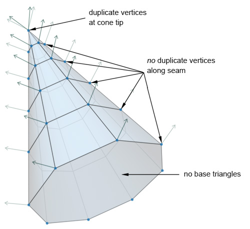
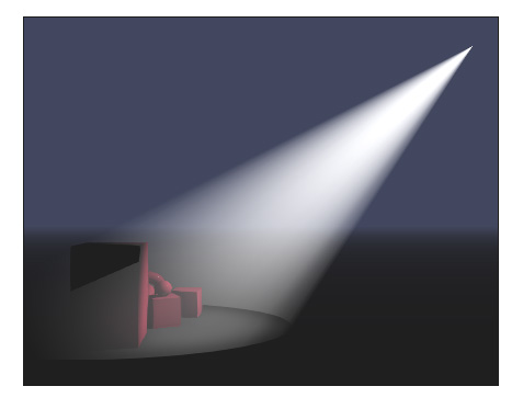
Global illumination (along with physically based rendering) is one of my favourite graphics areas and I don’t miss the opportunity to try new techniques every so often. One of my recent lunchtime experiments involved a quick implementation of Instant Radiosity, GI technique that can be used to calculate first bounce lighting in a scene, to find out how it performs visually.
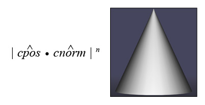
The idea behind Instant Radiosity is simple, cast rays from a (primary) light into the scene and mark the positions where they hit the geometry. Then for each hit sample the surface colour and add a new point light (secondary light, often called Virtual Point Light – VPL) at the collision point with that colour. The point light is assumed to emit light in a hemisphere centred on the collision point and oriented towards the surface normal. Various optimisations can be added on top like binning VPLs that are close together to reduce the number of lights.
Typically Instant Radiosity creates a large number of point lights, a situation not ideal for forward rendered scenes. On the other hand light-prepass engines (and deferred shading engines although in this case the bandwidth requirements might increase due to the larger G-Buffer) are much better suited to handle large numbers of lights, and such an engine (Hieroglyph to be more specific) I used for my quick implementation.
To determine light ray-surface collisions, one can use CPU raycasting or a compute shader based GPU solution like Optix. In this article the use of Optix is described in the context of a deferred lighting engine with very good results. In my case, I opted for a coarser but simpler solution to find the light ray/scene intersections which involved rendering the scene from the point of view of the light and creating two low resolution textures storing world positions (a cheated a bit here as I should really store normals) and surface colour. In essence, each texel stores a new VPL to be used when calculating scene lighting. This approach is in fact quite similar to the Reflective Shadowmaps technique, although in the context of the deferred lighting engine (in which lighting is done in one pass) I chose to store surface albedo and not surface radiance (or radiant flux as in the original paper).
For the purposes of my test, two 32×32 rendertargets storing world positions in the first and surface albedo on the second proved enough (resolution-wise). The following screenshot is the surface albedo as viewed from the directional light.
I am then feeding the two rendertargets as textures to the lighting pass shader directly to extract the Virtual Point Lights from. This has the advantage that I don’t have to read the textures back on the CPU to get the positions, gaining some performance increase. Hieroglyph performs lighting by calculating a quad for each light using a geometry shader and passing it to the pixel shader.
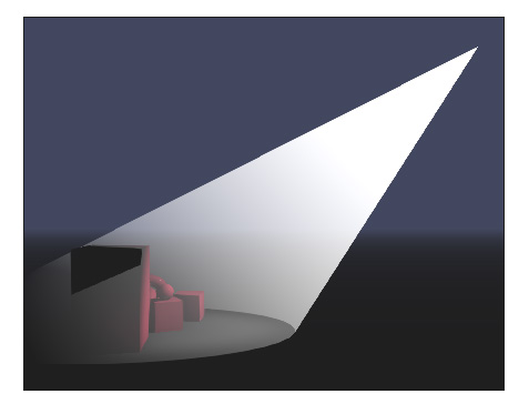
This is what the lightbuffer looks like after we render the bounced, point lights to it:
We can see the directional light being reflected from various surfaces, taking their albedo colour and lighting nearby objects.
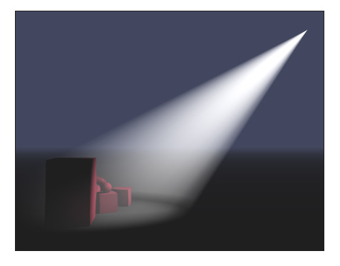
Finally we use the lightbuffer to light the scene:
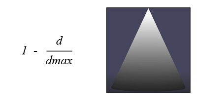
Once we add the surface albedo the bounced light colour becomes apparent. The radius of each VPL can be changed to cover more, or less area accordingly.
Moving the directional (primary) light does not seem to introduce any visible artifacts, although I’d imagine this is due to the low resolution of the reflective shadowmap, which means that VPLs are quite sparsely distributed.
This technique can be quite appealing as it is a straightforward way to add approximate first bounce lighting in a deferred, dynamically lit scene without adding any complexity, or actually modifying the lighting pass. There are some drawbacks; one, which is inherent to Instant Radiosity, is the fact that occlusion is not calculated for the VPLs meaning that light from the VPL can seem to penetrate a surface to reach areas that it shouldn’t. Determining occlusion for each VPL can be costly although it could probably be coarsely performed in screen space using the depth buffer. Directional and spot lights in the scene can easily be supported, not so for point lights which would require an onmi-directional shadowmap approach, or dual paraboloid shadowmaps to cover the whole scene. Coloured lights are not supported in this instance since I am storing surface albedo and not radiance. To achieve this would essentially require two lighting passes, one for the primary light and one for the VPLs. Finally the number of primary scene lights must be quite low (or one ideally) due to the number of prepasses required to calculate the reflective shadowmap for each.
This was a quite rushed implementation to get a feel of how the technique works. I’d definitely like to revisit in it the future and improve it by storing normals and depth instead of world positions (so that bounched lights can indeed be hemispheres) and maybe try other primary light types.
In the meantime, if anyone wants to have a go, here is the source code. You’ll have to install Hieroglyph to get it working.
Adaptive Volumetric Shadow Maps use a new technique that allows a developer to generate real-time adaptively sampled shadow representations for transmittance through volumetric media. This new data structure and technique allows for generation of dynamic, self-shadowed volumetric media in realtime rendering engines using today’s DirectX 11 hardware.
Each texel of this new kind of shadow map stores a compact approximation to the transmittance curve along the corresponding light ray. The main innovation of the AVSM technique is a new streaming compression algorithm that is capable of building a constant-storage, variable-error representation of a visibility curve that represents the light ray’s travel through the media that can be used in later shadow lookups.
Another exciting part of this sample is the use of a new pixel shader ordering feature found in new Intel® Iris™ and Intel® Iris™ Pro graphics hardware. Two implementations are provided in this sample - a standard DirectX implementation, and an implementation that utilizes this new graphics hardware feature.
This sample was authored by Matt Fife (Intel), Filip Strugar (Intel) with contributions from Leigh Davies (Intel), based on an original article and samplet from Marco Salvi (Intel).
A nice and cheap technique to approximate translucency was presented some time ago at GDC. The original algorithm depended on calculating the “thickness” of the model offline and baking it in a texture (or maybe vertices). Dynamically calculating thickness is often more appealing though since, as in reality, the perceived thickness of an object depends on the view point (or the light’s viewpoint) and also it is easier to capture the thickness of varying volumetric bodies such as smoke and hair.
An easy way to dynamically calculate thickness is render the same scene twice store the backfacing triangles’ depth in one buffer and the frontfacing ones’ in another and taking the difference of the values per pixel (implementing two-layer depth peeling in essence). This method works well but it has the disadvantage of rendering the scene at least one extra time.
Looking for ways to improve dynamic thickness calculation, I came across a dual depth buffering technique in ShaderX6 (“Computing Per-Pixel Object Thickness in a Single Render Pass” by Christopher Oat and Thorsten Scheuermann) which manages to calculate the thickness of an object/volume in one pass. The main idea behind this technique is to turn culling off, enable alpha blending by setting the source and destination blend to One and the blend operation to Min and store depth in the Red channel and 1-depth in the Green channel. That way we can calculate the thickness of an object in the main pass as thickness = (1 – Green) – Red. The depth can be either linear or perspectively divided (by w), although the latter will make the calculated thickness vary according to distance to the camera.
The following screenshots demonstrate this. The “whiter” the image the thicker it is. We can see that the thickness varies depending on the viewpoint (you can see that on the torso and the head for example)
This technique works nicely for calculating the thickness of volumetric bodies such as smoke and hair, but not that well for solid objects with large depth complexity as it tends to overestimate the thickness. You can see this in the above images (the leaves in front of the statue are very white) and the following couple of images demonstrate this problem in practice.
The model is rendered with the “fake” translucency effect mentioned above and by calculating the thickness dynamically with a dual depth buffer. We also placed a light source behind the statue. Viewing the statue from the front it looks ok and we can see the light propagating through the model at less thick areas (like the arm). If we rotate the statue so as to place the leaves between the body and the light we can see them through the statue (due to the overestimation of thickness it absorbs more light than it should and this areas appear darker).
This method is clearly not ideal for solid, complex, objects but we can modify slightly and improve it. Ideally I would like to know the thickness of the first solid part of the model as the ray travels from the camera into the scene.
So instead of storing (depth, 1-depth) in the thickness rendertarget for all rendered pixels I make a distinction between front facing the back facing samples and store the depth as such:
The blending mode remains the same (Min). This way I get the distance of the first front facing and the first backfacing triangle sample along the view ray and calculating the thickness is a matter of subtracting them: thickness = Green – Red.
The following two images demonstrate the effect:
The overall effect is the same as previously but now the leaves are no longer visible through the body of the statue since they are not taken into account when calculating the thickness at the specific pixels.
In summary, dual depth buffering is a nice technique to calculate the thickness of volumetric bodies and simple solid objects and with a slight modification it can be used to render more complicated models as well.
Today I am providing a small code snippet which I have found to be convenient.
Here is the header file: FilterBits.h
Here is the implementation: FilterBits.cpp
And if your compiler does not provide 'stdint.h' here is a link to a version of that include file: stdint.h
It is an extremely common use case in software development where you might want to define a collection of groups by name and give each group/property a representation as a bit in a bitmask integer value.
These flags are typically used to represent properties on an object, and one object might have multiple properties. You might have a set of bits which define what 'type' of object this is, and yet more bits that describe other properties of that object (friendly, enemy, or inside, outside, etc. etc.)
Often times you will have a set of bits which define the properties of an object and then another set of bits which describe which properties of another type of object this object reacts to. This is often used in 'collision filtering' where you take two objects and see if the filter bits match the type bits of another object. If they do, then you will treat the test as 'true' otherwise 'false'.
More complex boolean operations can be performed, but this is the common use case.
Now, here's the problem this code snippet is trying to solve. In almost all cases where a project needs to have a set of bitfields, representing properties on an object, those bitfields are hard-coded and predefined in the source code. Usually with an enumerated type or some defines.
However, if you want to make a general purpose property system, that is not hard coded, this doesn't really map very well.
This code snippet lets an artist/designer decide which 'object types' there are. It's completely up to them, so long as they don't create more than the maximum number of 64 unique types, it is fine.
The provided sample code will parse the input types and convert it to a bit-pattern that you can use in C++.
Personally, I have found this to be a useful and valuable tool.
There are two reserved 'types'. They are the type 'all' and 'none'; meaning exactly what you think they would mean.
For example, the artist/designer might define a string like:
Player,Enemy=All
Which could be interpreted as meaning this is a player, and an enemy, that interacts with 'all' other types of objects.
This code converts the input string in the form of: "a,b,c=d,f,g" into a 64 bit source bit pattern and a corresponding 64 bit destination bit pattern.
The returned bit patterns are guaranteed to be persistent, that the the application can cache them for future use and does not need to ever have them regenerated.
If you don't need 64 bits and only 32, then there are accessor methods which will return the results as two 32 bit numbers instead.
The intended use of this snippet is so you can allow artists/designers to create a set of arbitrary ASCII strings which represent the properties pair, defining type and interaction, in some kind of editing tool. At run-time your code just passes in the string on startup and gets back the run-time binary code which is all you use from that point forward (i.e. don't convert the strings to bitmasks every time you want to use them.)
For OpenGL Insights, we created an OpenGL 4.2 and OpenGL ES 2.0 pipeline map.
Patrick Cozzi asked me few times to update it for OpenGL 4.3 and OpenGL ES 3.0 but obviously I found interest in making it only to make it a lot more detailled
considering that it would not be for printing so it could be as big as I see fit. This endeavour represented a significant amount of work but finally I have completed the OpenGL 4.3 Pipeline Map.
Wonder why Larrabee for graphics failed? I guess when we see all this fixed function functionalities that hardware vendor can implement very effectively, it gives us some clues.
Mola, un prng al con el que puedes ir hacia adelante y hacia atrás :D:D
It isn’t very often that you need a pseudo random number generator (PRNG) that can go forwards or backwards in time, or skip to specific points in the future or the past. However, if you are ever writing a game like Braid and do end up needing one, here’s one way to do it.
At the core of how this is going to work, we are going to keep track of an index, and have some way to convert that index into a random number. if we want to move forward in time, we will just increment the index. If we want to move backwards in time, we will just decrement the index. It’s super simple from a high level, but how are we going to convert an index into a random number?
There are lots of pseudo random number generators out there that we could leverage for this purpose, the most famous being C++’s built in “rand()” function, and another one famous in the game dev world is the Mersenne Twister.
I’m going to do something a little differently though as it leads well into the next post I want to write, and may be a little bit different than some people are used to seeing; I want to use a hash function.
Murmur Hash 2
Good hash functions have the property that small changes in input give large changes in output. This means that if we hash the number 1 and then hash the number 2, that they ought not to be similar output, they ought to be wildly different numbers in the usual case. Sometimes, just like real random numbers, we might get 2 of the same numbers in a row, but that is the desired behavior to have the output act like real random sequences.
There are varying levels of quality of hash functions, ranging from a simple string “hash” function of using the first character of a string (super low quality hash function, but super fast) all the way up to cryptographic quality hash functions like MD5 and SHA-1 which are a lot higher quality but also take a lot longer to generate.
In our usage case, I’m going to assume this random number generator is going to be used for game use, where if the player can discover the pattern in the random numbers, they won’t be able to gain anything meaningful or useful from that, other than at most be able to cheat at their own single player game. However, I really do want the numbers to be fairly random to the casual eye. I don’t want visible patterns to be noticeable since that would decrease the quality of the gameplay. I would also like my hash to run as quickly as possible to keep game performance up.
Because of that level of quality I’m aiming for, I opted to go with a fast, non cryptographic hash function called Murmur Hash 2. It runs pretty quick and it gives pretty decent quality results too – in fact the official Murmur Hash Website claims that it passes the Chi Squared Test for “practically all keysets & bucket sizes”.
If you need a higher quality set of random numbers, you can easily drop in a higher quality hash in place of Murmur Hash. Or, if you need to go the other way and have faster code at the expensive of random number quality, you can do that too.
Speed Comparison
How fast is it? Here’s some sample code to compare it vs C++’s built in rand() function, as well as an implementation of the Mersenne Twister I found online that seems to preform pretty well.
#include <stdio.h>
#include <stdlib.h>
#include <time.h>
#include <windows.h>
#include "tinymt32.h" // from http://www.math.sci.hiroshima-u.ac.jp/~m-mat/MT/TINYMT/index.html

// how many numbers to generate
#define NUMBERCOUNT 10000000  // Generate 10 million random numbers

// profiling macros
#define PROFILE_BEGIN \
{ \
	LARGE_INTEGER freq; \
	LARGE_INTEGER start; \
    QueryPerformanceFrequency(&freq); \
    QueryPerformanceCounter(&start); \

#define PROFILE_END(label) \
	LARGE_INTEGER end; \
	QueryPerformanceCounter(&end); \
	printf(label " - %f ms\r\n", ((double)(end.QuadPart - start.QuadPart)) * 1000.0 / freq.QuadPart); \
}

// MurmurHash code was taken from https://sites.google.com/site/murmurhash/
//-----------------------------------------------------------------------------
// MurmurHash2, by Austin Appleby

// Note - This code makes a few assumptions about how your machine behaves -

// 1. We can read a 4-byte value from any address without crashing
// 2. sizeof(int) == 4

// And it has a few limitations -

// 1. It will not work incrementally.
// 2. It will not produce the same results on little-endian and big-endian
//    machines.

unsigned int MurmurHash2 ( const void * key, int len, unsigned int seed )
{
	// 'm' and 'r' are mixing constants generated offline.
	// They're not really 'magic', they just happen to work well.

	const unsigned int m = 0x5bd1e995;
	const int r = 24;

	// Initialize the hash to a 'random' value

	unsigned int h = seed ^ len;

	// Mix 4 bytes at a time into the hash

	const unsigned char * data = (const unsigned char *)key;

	while(len >= 4)
	{
		unsigned int k = *(unsigned int *)data;

		k *= m;
		k ^= k >> r;
		k *= m;

		h *= m;
		h ^= k;

		data += 4;
		len -= 4;
	}

	// Handle the last few bytes of the input array

	switch(len)
	{
	case 3: h ^= data[2] << 16;
	case 2: h ^= data[1] << 8;
	case 1: h ^= data[0];
	        h *= m;
	};

	// Do a few final mixes of the hash to ensure the last few
	// bytes are well-incorporated.

	h ^= h >> 13;
	h *= m;
	h ^= h >> 15;

	return h;
}

void RandTest()
{
	for(int index = 0; index < NUMBERCOUNT; ++index)
		int i = rand();
}

unsigned int MurmurTest()
{
	unsigned int key = 0;
	for(int index = 0; index < NUMBERCOUNT; ++index)
		key = MurmurHash2(&key,sizeof(key),0);
	return key;
}

// g_twister is global and inited in main so it doesnt count towards timing
tinymt32_t g_twister;
unsigned int TwisterTest()
{
	unsigned int ret = 0;
	for(int index = 0; index < NUMBERCOUNT; ++index)
		ret = tinymt32_generate_uint32(&g_twister);
	return ret;
}

int main(int argc, char**argv)
{
	// rand() test
	PROFILE_BEGIN;
	RandTest();
	PROFILE_END("rand()");

	// hash test
	unsigned int murmurhash;
	PROFILE_BEGIN;
	murmurhash = MurmurTest();
	PROFILE_END("Murmur Hash 2");

	// twister test
	g_twister.mat1 = 0;
	g_twister.mat2 = 0;
	tinymt32_init(&g_twister, 0);
	unsigned int twister;
	PROFILE_BEGIN;
	twister = TwisterTest();
	PROFILE_END("Mersenne Twister");

	// show the results
	system("pause");

	// this is here so that the murmur and twister code doesn't get optimized away
	printf("%u %u\r\n", murmurhash, twister);

	return 0;
}
Here’s the output of that code run in release on my machine, generating 10 million random numbers of each type. You can see that murmurhash takes about 1/3 as long as rand() but is not quite as fast as the Mersenne Twister. I ran this several times and got similar results, so all in all, Murmur Hash 2 is pretty fast!
Final Code & Sample Output
Performance looks good but how about the time traveling part, and how about seeing some example output?
Here’s the finalized code:
#include <stdio.h>
#include <stdlib.h>
#include <time.h>
// MurmurHash code was taken from https://sites.google.com/site/murmurhash/
//-----------------------------------------------------------------------------
// MurmurHash2, by Austin Appleby
// Note - This code makes a few assumptions about how your machine behaves -
// 1. We can read a 4-byte value from any address without crashing
// 2. sizeof(int) == 4
// And it has a few limitations -
// 1. It will not work incrementally.
// 2. It will not produce the same results on little-endian and big-endian
// machines.
unsigned int MurmurHash2 ( const void * key, int len, unsigned int seed )
{
// 'm' and 'r' are mixing constants generated offline.
// They're not really 'magic', they just happen to work well.
const unsigned int m = 0x5bd1e995;
const int r = 24;
// Initialize the hash to a 'random' value
unsigned int h = seed ^ len;
// Mix 4 bytes at a time into the hash
const unsigned char * data = (const unsigned char *)key;
while(len >= 4)
{
unsigned int k = *(unsigned int *)data;
k *= m;
k ^= k >> r;
k *= m;
h *= m;
h ^= k;
data += 4;
len -= 4;
}
// Handle the last few bytes of the input array
switch(len)
{
case 3: h ^= data[2] << 16;
case 2: h ^= data[1] << 8;
case 1: h ^= data[0];
h *= m;
};
// Do a few final mixes of the hash to ensure the last few
// bytes are well-incorporated.
h ^= h >> 13;
h *= m;
h ^= h >> 15;
return h;
}
class CReversablePRNG
{
public:
CReversablePRNG()
{
m_index = 0;
m_seed = 0;
}
unsigned int NextNumber()
{
unsigned int ret = MurmurHash2(&m_index, sizeof(m_index), m_seed);
m_index++;
return ret;
}
unsigned int LastNumber()
{
unsigned int lastIndex = m_index - 2;
unsigned int ret = MurmurHash2(&lastIndex, sizeof(lastIndex), m_seed);
m_index--;
return ret;
}
// to be able to save / restore state for a save game or whatever else
void GetState(unsigned int &index, unsigned int &seed)
{
index = m_index;
seed = m_seed;
}
void SetState(unsigned int index, unsigned int seed)
{
m_index = index;
m_seed = seed;
}
private:
unsigned int m_index;
unsigned int m_seed;
};
int main(int argc, char**argv)
{
// create and seed our random number generator. If two similar numbers are hashed
// they should give very different results usually, so for a seed, we can hash the
// time in seconds, even though the number from run to run should be really similar
CReversablePRNG prng;
unsigned int currentTime = time(NULL);
unsigned int seed = MurmurHash2(¤tTime, sizeof(currentTime), 0x1337beef);
prng.SetState(0, seed);
// display our seed and our table header
printf("seed = %u\r\n", seed);
printf("index | raw number | mod 10\r\n");
printf("---------------------------\r\n");
// generate 10 numbers forward
for (int index = 0; index < 10; ++index)
{
unsigned int nextNumber = prng.NextNumber();
printf("%2i | %10u | %u\r\n", index, nextNumber, nextNumber % 10);
}
// generate 3 numbers back
printf("\r\n");
for (int index = 0; index < 3; ++index)
{
unsigned int lastNumber = prng.LastNumber();
printf("%2i | %10u | %u\r\n", 8 - index, lastNumber, lastNumber % 10);
}
// generate 5 numbers forward
printf("\r\n");
for (int index = 0; index < 5; ++index)
{
unsigned int nextNumber = prng.NextNumber();
printf("%2i | %10u | %u\r\n", 7 + index, nextNumber, nextNumber % 10);
}
system("pause");
return 0;
}
"I'm making it free because Linux users are such strong supporters of indie games and because I like Linux, and the philosophy behind it so much," Colin Northway wrote in. Linux is an open source operating system that is a viable alternative to Windows and Mac OS X. On the non-sales page, the developer explains how to get started using Linux.
Incredipede is also discounted via the Humble Store widget for Windows and Mac, with 50% of profits going to two open source projects Colin used in making his game: FlashDevelop and Box2d.
Lastly in the world of halves, the Steam version is 50% off, too. It's a full-on assault from Quozzle!
Unlike many programmers, I actually prefer to use one monitor these days. A lot of my colleagues have Visual Studio filling the entirety of their primary monitor and either Outlook or documentation filling the other, often with a bunch of other apps like Lync, a command prompt or two, and likely a music player.
When I moved to Microsoft HQ about 5 months ago I found that my new PC was lacking a second HDMI output and I didn’t have a DVI-VGA converter for the second twenty-something inch monitor I’d been given. Weirdly, once the part arrived a week or so later, I went to plug it in and… found that I didn’t want to.
A single monitor really cut down the distractions. I get a lot of mail – a lot of mail – and the constant flood of it in the corner of my eye was becoming a problem. (I have to add that turning off the task-bar’s “New Mail” icon in Outlook also helped a lot.)
Since I cut down to a single screen, my ability to focus has increased dramatically and that my primary monitor is easily big enough for code and documentation if the need arises. I actually prefer having the documentation right there, next to my code, rather than having to flick my eyes over to another monitor.
When I need to “dual wield”, I use the little known Windows key + Arrow keys hotkeys. If you’re unfamiliar with these, give them a try. Windows+Left and Windows+Right are by far the most useful, as they will:
snap the window to the left or right half of the screen,
flip the window onto the next monitor if you have one.
Windows+Up will maximize, whereas Windows+Down will restore or minimize depending on the window’s current state.
After about 5 months of using them, these shortcuts are now indispensable. However, they weren’t quite useful enough. A common scenario is that I just want a little more than half the screen for code, as documentation pages tend to deal well with smaller browser sizes. Or, sometimes I have a command prompt pinned to the right, but I have to fiddle about with the mouse to fill the gap because command windows won’t generally expand horizontally.
Another problem was stacking windows above each other. In an ideal world, VS would occupy 60% of the left side of my monitor, and on the remaining right side, I’d have documentation taking 70% of the top right corner and the command prompt in the bottom right 30%. With the vanilla Windows hotkeys, this is impossible with keyboard alone.
And thus, my answer to this was to write code, culminating in this: Advanced Window HotKeys. This is a tiny app that will run in the background, and using the Alt+Arrow keys (among others) will net you some really fine-grained control over your window layout. I went one step further and the tool will also help you preserve your current layout but still allow you to resize the foreground window, moving other windows out of the way. Check out the page for more information.
I wrote this in VS2012, C++ and Win32. Win32 really is a very powerful API. This tool makes extensive use of EnumWindows and MoveWindow to expand or contract the foreground window; search for adjacent windows to snap to; modify adjacent windows to prevent overlap;and other stuff. I threw in a little Control Panel, although that’s still very primitive.
I haven’t tested this on anything other than Win8, so if anyone wants to volunteer to see how this’ll work on Win7 or below then please comment or email me. I’d really appreciate feedback, so you can do that using the email link at the bottom of the AWHK website.
The Binary EZ-Mesh file reader project, tools, and documentation can be found at the following Google Code project.
Quite some time ago I created a graphics file format that I call 'EZ-Mesh'. My design goal was to create an extremely 'easy' way to represent 3D graphics data without requiring a massive amount of source code or bloated API.
Originally the file representation for this data was always in XML but, as we all know, XML can get pretty bloated and take some time to parse. We are currently using EZ-Mesh in a bunch of our APEX SDK samples at NVIDIA; specifically all of our clothing samples. We have some very high poly count samples for clothing in the APEX SDK and needed to load them on consoles and tablets. Parsing massive XML files did not seem like the way to go; so thus was born the binary EZ-mesh format.
Below is a short video sample of a character being mocked up with clothing for the APEX SDK
The artists work in 3D Studio Max and Maya, but the goal for the programmer is to get the relevant data out of there and into our samples.
Now, Autodesk provides a file format and SDK to do this. It's called the 'FBX' file format. However, to access the data in an .FBX file requires using a very large SDK and API. This API is really huge and complex and, of course, isn't likely to run in real-time on a console or tablet device.
So, our need was a way to extract the relevant data from an .FBX file (meshes, materials, skeletons, and animation data) and convert it into something very simple that we could load directly into our samples.
That's where EZ-Mesh comes in and the project I'm presenting today.
When you sync to this project you will get a pre-built tool called 'MeshConvert', and a D3D9 viewer application called 'CodeSuppository'; as well as full source to a very tiny project that can read the contents of a binary EZ-Mesh into your own application.
This project has an extensive ReadMe.txt file as well as source code documentation, so I won't go into all of the details here.
The quick summary is that with the provided tool, you can convert a wide variety of graphics formats, including FBX, Ogre3d, UE3 PSK, and some others, into EZ-Mesh either XML or binary format.
The conversion tool also has some command line switches that allow you to scale or rotate the input mesh before it is saved back out again. The conversion tool can also export several different graphics file formats in addition to EZ-Mesh.
You can use the 'CodeSuppository' viewer app to preview the files.
The 'EZ-Mesh' format is defined in a single header file 'EZMesh.h' which is a completely flat set of data structures contains mesh data, vertex buffers, index buffers, skeletons, and animation data.
There is *no* API whatsoever!! It's just a straight flat data structure that you can easily iterate through.
It is important to note that the EZ-Mesh data layout is *not* meant to be a production format. It's sole purpose is to provide an extremely easy to access flat layout for raw mesh, skeleton, and animation data. The purpose was not to be memory efficient.
If you are writing a small sample and just want to quickly load a 3D graphics file with skeletons and animation data, then EZ-Mesh is for you. You can also use it as an intermediate format as part of a tool chain to ultimately convert the data into some final project ready format of your own choosing.
The EZ-Mesh source code uses the PhysX/APEX SDK 'foundation' header files. These header files just define very simple and basic platform agnostic data types; such as defining floats and integers of various bit sizes and a basic set of vector classes.
I do not have permission to redistribute the PhysX SDK foundation header files so what I have done with this open source project is created very simple proxy placeholders.
It is recommended that you either get the actual header files from the PhysX SDK or do a global find replace on the source to remap the data types to whatever your project prefers to use.
I have *not* included full source code to the mesh converter tool, import/export DLL plugins, or the viewer app. That was out of scope for this article today.
You only need three source files (not counting the foundation headers) to load a binary EZ-Mesh into your application in a format ready for you to process, render, animate, etc.
The first is: 'EZmesh.h' which simply defines the flat data structures containing the mesh data. As stated before, it has no API and no dependencies other than the foundation primitive types.
Next is: 'MeshImportEZB.h' which simply declares the API to parse a binary EZ-mesh blob into the data structure.
Finally is: 'MeshImportEZB.cpp' which contains the implementation to parse the binary EZ-mesh file, and to release temporary memory allocated when you are finished with it. This source has no dependencies on the STL, Windows, or anything else. In theory is should easily compile on almost any platform available; and it takes endian specific issues into account. In fact, the binary EZ-mesh format defaults to big-endian format just so that it will load a little bit faster on some console platforms.
'MeshImportEZB.cpp' is just a little over 700 lines of code for the whole thing. The source comes with two *exporters* simply so you can step through the code and see how the various data structures are accessed. It also acts as a validation test for the importer.
My design goal was to provide a tool chain that would produce a binary file containing all relevant 3D graphics data that could be loaded quickly and easily into a sample project.
I think I have accomplished that goal, let me know if you find any of this useful.
It’s that time of the year again, when everyone else is partying and having fun (or maybe not – WTF IGDA?) at GDC in San Francisco. I’ll try to collect any links to lecture materials I come across. If you know of stuff missing here, please tell me about it on Twitter @TheJare. You can also check industry sites like Gamasutra, Polygon or Develop for ongoing coverage, and hopefully a lot of these materials will show up in the GDC Vault soon.
Como dice wisefox, han pasado 20 años desde que se inventó el fuego :)
It’s been nearly 20 years since we released that old fire effect and the demoscene turned out to love it. I have ported it to HTML5 to celebrate!
It all started when we bought a math coprocessor for our 386/25 and I started playing with fractals and plasmas. A few programming mistakes later, this thing came out and looked neat, so we slapped JCAB’s VT player and released it. Eternal gratitude to Jester of Sanity for unknowingly lending me his fantastic ‘Elysium’ mod – it didn’t take me long to learn that such acts were VERY badly frowned upon.
You can check out the source code on github if you are so inclined. The comments are slightly better this time! This version runs rather slowly on Chrome, and I don’t really know why, but IE, Firefox (Win and Android) and iOS Safari work great.
I have implemented a simple idea on how one can render real-time single scattering in participating medias with relative small effort and cost. This can be used to simulate e.g. the effect of light bleeding through objects. The idea combines the depth information obtained from a shadow map and a depth-peeling rendering. Consider an object/media as depicted below.
The problem we want to address is how much light going is going in the direction of the eye/camera. From the rendering equation of participating medias we limit the lighting model to the following contributions to the radiance arriving at the eye,
Here is the ordinary scattering of light at the surface point A, is the light which arrives at the backside surface point B of the object and is attenuated through the media due to scattering, and finally is the radiance arriving through the media from the light source along the line of sight inside the object (e.g. point C) and scattered in the direction of the eye.
When rendering the scene we will have access to the information at point A in the fragment shader and can implement e.g. a Blinn–Phong shading for the or any other model that suits our needs. In order to obtain the we will need besides a rendering of the scene without the object, the thickness of the object along the line of sight, since the attenuation through the media is essentially just exponentially damped. To obtain this thickness we must have access to the next-nearest depth value which can be obtained by using a depth-peeling scheme. Think of it as a depth buffer storing the depth of the surface behind the nearest. Attaching this next-to-nearest depth buffer to the fragment shader we have access to the thickness of the object along the line of sight, that is the distance |AB|. What this term achieves is essentially just an alpha blending with varying alpha value across the surface.
Thanks to Humus for providing the skybox texture
Now, in order to compute the contribution we will need to know the distance |Cc| from any point C along the line of sight inside the object to the boundary of the object (point c) in the direction of the light source. All this information is stored in the shadow map, but in particular, we can look up the depth distances from the light source to the object in the direction of the points A and B, that is the distance from the light source to a and b. Having the positions of those two points in the shadow map one can integrate/sample the linear path between the two points while having access to all distances from the light source to the object in the direction of any point on the line of sight. This integration can be approximated in many ways, but the simplest is to assume that one can do a linear interpolation of the values across the line inside the object, so simply using the depth values at the two end points A and B. In this case one can perform the integrations analytically assuming that the scattering coefficients are constant throughout the object and that the phase function is simple e.g. uniform scattering, that is constant and equal to 1/4pi. Also, one can to good approximation neglect that the "rays" are refracted at the boundaries of the object.
And of course we need a rendering of the cornell box with some not so realistic shadows for the translucent object, but hey, they come for free, since we have generated the shadow map.
The current state of competitive, skilled FPS games is a topic that comes up often in discussions among my game industry friends, with players and with anyone involved with eSports.
There is lament that no FPS title has been able to grow a big enough audience and pull enough weight around to be represented on the major circuits like MLG or ESL recently. There are a lot of ins and outs to that discussion, but one aspect that is of particular interest to me is the projects that are at various stages of development, trying to crack that nut and make it big for an eSport FPS title again.
I need to mention a few of those to ground the discussion a bit. QuakeLive is the old guard, it's still around and kicking, surprisingly resilient etc. Then there are newer, more active titles, like CS:GO and Shootmania. Further down on the horizon there's rumored projects like James Harding's Reborn.
This got me thinking about how I would approach this, and what my ideal engine framework would look like. We are talking PC-centric, mouse and keyboard gaming here. High end GPU, multicore CPU, 120 Hz display and low latency, high precision input.
Renderer eye candy should never get in the way of a smooth game simulation. A sudden dip in renderer fps should never mean that you are going to miss that jump, or that your mouse handling is going to turn you around in a slightly different way than usual.
The technology foundation for a project like this is extremely important. Unity and UDK are amazing engines, but they are general purpose in nature, and they made compromises to that end which make them ill-suited.
So I decided to put some code together to explore the subject. There's just enough stuff now that I feel it's worth putting it out to get some feedback. I've named this es_core, you can find the project on github.
And now I'll just ramble on about what's in the code. I picked Ogre as the renderer, it's a simple API, great cross platform support, and for the most part it only cares about doing rendering. I went to SDL2 for window creation, rendering context setup and input management.
The input is sampled in a dedicated thread, and input state is made available to the game thread or the render thread with a reply/request system. Polling for input on a dedicated thread makes this independent from game logic or renderer timings, which is a big step towards responsive and consistent control.
The threads communicate with each other through message passing only. That system is built on ZeroMQ, a design for which Pieter Hintjens makes a very convincing argument in this article. There is more work in that area: building an efficient binary protocol instead of the current text protocol (I am considering Cap'n Proto), and optimizing the code to use zero-copy message transfers, removing all memory heap operations.
Now to the game and render threads. The game logic runs at a fixed tick (60Hz atm) and updates an internal game state. It produces a new render state with each tick, which is forwarded to the render thread. The renderer runs at the display refresh rate and interpolates between the two most recent render states. There is a great piece by Glenn Fiedler about this approach.
I wanted a small demo to show those pieces working together, but I didn't want to put in any kind of game design, by fear that it would distract from the subject matter. So all you get for now is a head bouncing about that can be spun around with mouse drags. For the most part, writing this was a refreshing exercise on Quaternion math. The demo shows how input can be used by the game thread for general logic and directly by the render thread for smoother, low latency control.
The next big step will be the addition of networked multiplayer. There will probably be another big post like this when that comes together. My current line of thought is that the architecture of the game code should be driven by the needs of the network system, and not the other way around.
This work is a fun side project for me. I'm only giving it a few hours here and there as time and energy permits. It's a great feeling to use all this technology and stand on the shoulders of giants to make new things.
ale, como todo el mundo tiene deferreds ya, esto es facilote facilote :D
Originally posted on 06/01/2012
Volumetric effects are one of the perennially tricky problems in realtime graphics. They effectively simulate the scattering of light through particles suspended in the air. Since these effects can enhance both the realism and aesthetic appearance of a rendered scene, it would be nice to have a method which can produce "good enough" results cheaply and simply. As the title implies, "good enough" is the main criteria here; we're not looking for absolute photorealism, just something that's passable which adds to the aesthetic or the mood of a scene without costing the Earth to render.
I'll be describing a volumetric effect for spot lights, although the same ideas will apply to other types lights with different volume geometries.
Coneheads
The volume affected by a spotlight is a cone, so that's what we'll use as the basis for the technique. How you generate the cone is up to you, but it must have per-vertex normals (they'll make life easier later on), no duplicated vertices except at the cone's tip and no base. I've found that having plenty of height segments is good for the normal interpolation and well worth the extra triangles.
The basic idea is to render this cone in an additive blending pass with no face culling (we want to see the inside and outside of the cone together), with depth writes disabled but the depth test enabled. As the screenshot below shows, on its own this looks pretty terrible:
Attenuation
To begin to improve things we need to at least attenuate the effect along the length of the cone. This can be done per-fragment as a simple function of the distance from the cone's tip (d) and some maximum distance (dmax):
Already things are looking a lot better:
Soft Edges
The edges of the cone need to be softened somehow, and that's where the vertex normals come in. We can use the dot product of the view space normal (cnorm) with the view vector (the normalised fragment position, cpos) as a metric describing how how near to the edge of the cone the current fragment is.
Normalising the fragment position gives us a vector from the eye to the point on the cone (cpos) with which we're dealing. We take the absolute value of the result because the back faces of the cone will be pointing away but still need to contribute to the final result in the same was as the front faces. For added control over the edge attenuation it's useful to be able to raise the result to the power n.
Using per-vertex normals like this is simple, but requires that the cone geometry be set up such that there won't be any 'seams' in the normal data, hence my previous note about not having any duplicate vertices except at the cone's tip.
One issue with this method is that when inside the cone looking up towards the tip the normals will tend to be perpendicular to the view direction, resulting in a blank spot. This can be remedied by applying a separate glow sprite at the light source position.
Soft Intersections
As you can see in the previous screenshot there is a problem where the cone geometry intersects with other geometry in the scene, including the floor. Remedying this requires access to the depth buffer from within the shader. As the cone's fragments get closer to fragments already in the buffer (i.e. as the difference between the depth buffer value and the cone fragment's depth approaches 0) we want the result to 'fade out':
The result should be clamped in [0, 1]. The radius can be set to make the edges softer or harder, depending on the desired effect and the scale of the intersecting geometry compared with the cone's size. This does produce a slightly unusual fogging effect around the cone's boundary, but to my eye it meets the "good enough" criteria.
Another issue is that the cone geometry can intersect with the camera's near clipping plane. This results in the effect 'popping' as the camera moves across the cone boundary. We can solve this in exactly the same way as for geometry intersections; as the cone fragment's depth approaches the near plane we fade out the result.
 Want to go off-road? This jam-packed tutorial offers C++ code snippets for simulating water, mud, and different lighting conditions in a natural driving environment. ...


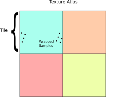
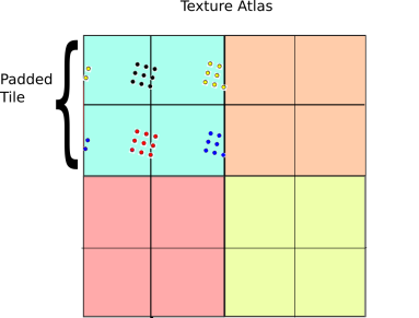
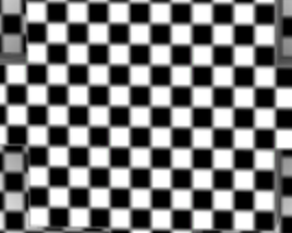

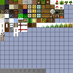 Base Tilesheet


 Some things to try out in the demo are displaying the wireframes and changing the mip map filtering mode when zooming and zooming out. The controls for the demo are:
 Having trouble getting your terrain textures to blend properly? This short tutorial, with code samples, will put you on track. ...

 ) reflection effects.


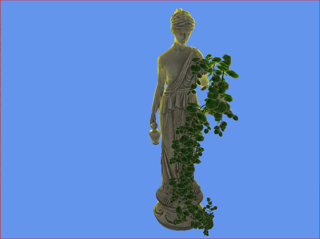


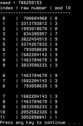
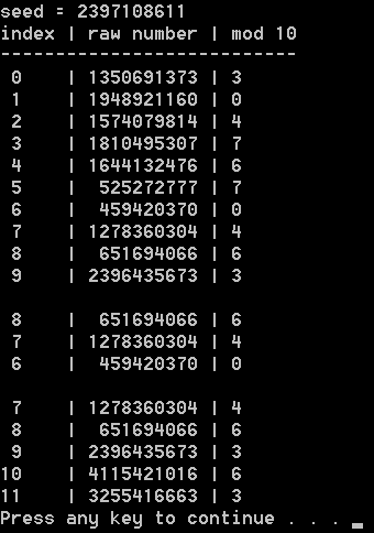
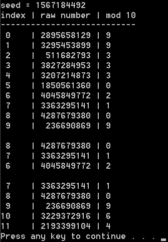
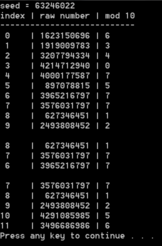
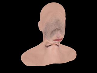

 Today's a great day to become a Linux user. Northway Games' gorgeous, lively physics puzzler Incredipede is now available on Linux for free.


 is the ordinary scattering of light at the surface point A,
  is the light which arrives at the backside surface point B of the object and is attenuated through the media due to scattering, and finally
  is the radiance arriving through the media from the light source along the line of sight inside the object (e.g. point C) and scattered in the direction of the eye.
  contribution we will need to know the distance |Cc| from any point C along the line of sight inside the object to the boundary of the object (point c) in the direction of the light source. All this information is stored in the shadow map, but in particular, we can look up the depth distances from the light source to the object in the direction of the points A and B, that is the distance from the light source to a and b. Having the positions of those two points in the shadow map one can integrate/sample the linear path between the two points while having access to all distances from the light source to the object in the direction of any point on the line of sight. This integration can be approximated in many ways, but the simplest is to assume that one can do a linear interpolation of the values across the line inside the object, so simply using the depth values at the two end points A and B. In this case one can perform the integrations analytically assuming that the scattering coefficients are constant throughout the object and that the phase function is simple e.g. uniform scattering, that is constant and equal to 1/4pi. Also, one can to good approximation neglect that the "rays" are refracted at the boundaries of the object.