Shared posts

16 Feb 11:12

The useful functions for modern OpenGL 4.4 programming

If anything, at least Mantle created some discussions about graphics API but it remains that I believe it's a waste of AMD engineering resources that could have benefit their OpenGL drivers for example.

Looking at the published list of Mantle functions, Mantle API looks really thin compared to OpenGL API for example. However, Mantle targets only AMD Southern Islands onward, while OpenGL 4.4 core profile targets all OpenGL 3 / Direct3D 10 and OpenGL 4 / Direct3D 11 GPUs. If we consider OpenGL 4.4 compatibility profile, then the API covers all GPUs even made.

Let's compare what we can compare. What if we want to write a Modern OpenGL program for AMD Southern Islands and NVIDIA Kepler only. Then we only need a tiny subset of the OpenGL API that I have listed below.

It still appears that Mantle requires less functions. With a closer look we see that Mantle use state objects to group rasterizer, viewport, depth test states. State objects are a idea because every hardware vendor would want different packing but also because every single OpenGL program would use different packing. To write an efficient OpenGL renderer we need to consider the update frequences and move every operations at the lower update rate possible. Packing states is requiring to update more often states that should not have change hence adding CPU overhead. So no thank you but I prefer to have no state object. However, what worked for me in the past (about 2007) was to use display lists to create immutable state objects that matched my program needs. I don't think I want to go this way in 2014.

So OpenGL has evolved, "revolution through evolution". If we really want to write low overhead OpenGL programs, we can. If that's not the case right now, my opinion is that the industry didn't put the effort in it because it has higher priority issues to resolve, essentially production issues which include supporting old consoles (PS3 and XBox, OpenGL 2.1 / Direct3D 9 hardware), cross compiling shaders, the development of mobile and the rise of WebGL.

Reflexion API (only for tools developers):
16 Feb 11:12

Large-Scale Liquid Simulation on Adaptive Hexahedral Grids

by christopherbatty

Florian Ferstl, Rudiger Westermann, Christian Dick

Regular grids are attractive for numerical fluid simulations because they give rise to efficient computational kernels. However, for simulating high resolution effects in complicated domains they are only of limited suitability due to memory constraints. In this paper we present a method for liquid simulation on  an adaptive octree grid using a hexahedral finite element discretization, which reduces memory requirements by coarsening the elements in the interior of the liquid body. To impose free surface boundary conditions with second order accuracy, we incorporate a particular class of Nitsche methods enforcing the Dirichlet boundary conditions for the pressure in a variational sense. We then show how to construct a multigrid hierarchy from the adaptive octree grid, so that a time efficient geometric multigrid solver can be used. To improve solver convergence, we propose a special treatment of liquid boundaries via composite finite elements at coarser scales. We demonstrate the effectiveness of our method for liquid simulations that would require hundreds of millions of simulation elements in a non-adaptive regime.

Large-Scale Liquid Simulation on Adaptive Hexahedral Grids

14 Feb 16:40

Functional Data Structures in C++: Lists

by Bartosz Milewski
“Data structures in functional languages are immutable.” What?! How can you write programs if you can’t mutate data? To an imperative programmer this sounds like anathema. “Are you telling me that I can’t change a value stored in a vector, delete a node in a tree, or push an element on a stack?” Well, yes […]
14 Feb 09:52

Car Make and Model Recognition using 3D Curve Alignment

We present a new approach for recognizing the make and model of a car from a single image. While most previous methods are restricted to fixed or limited viewpoints, our system is able to verify a car's make and model from an arbitrary view. Our model consists of 3D space curves obtained by backprojecting image curves onto silhouette-based visual hulls and then refining them using three-view curve matching. We also build an appearance model of taillights which is used as an additional cue. Our approach is able to verify the exact make and model of a car over a wide range of viewpoints and background clutter. This technical report describes research done during Edward Hsiao's summer internship at Microsoft Research in 2011 and was authored during the fall of 2011. A conference version of this work, presented at WACV 2014 [Ramnath et al., WACV 2014], contains newer pose estimation techniques and updated experimental results, but not some of the appearance-based matching described in this report. The two appendices in this report are new and provide additional details on the pose estimation component and additional experimental results relating to [Ramnath et al., WACV 2014].
14 Feb 09:52

Steam Dev Days talk posted

The slides and video of my talk from Steam Dev Days has been posted. It's basically the Haswell refresh (inside joke) of my SIGGRAPH talk from last year.

12 Feb 15:49

Brackets Sprint 36 Build

by Kevin Dangoor

The New Year is here, and we’ve got a new Brackets build for you. OK, so we’re actually a few days past the Chinese New Year, but the new Brackets build is all the more awesome as a result.

We’ve got two infrastructure improvements that will enhance your day-to-day use of Brackets and a variety of other additions that we think you’ll like.

Faster Files

We landed a major infrastructure change in Brackets 36: file watchers with caching. You’ll notice this change when you alter files and folders outside of Brackets and the Brackets project tree updates right away without you having to “refresh” it. The new caching layer makes repeated use of the “Find in Files” command much faster because the files are read from the cache the second time around.

Preferences for your Projects

The Brackets preferences system has been overhauled, opening the door to a wider variety of customization options for Brackets.

With Brackets 36, you can create a .brackets.json file in the top directory of your project. When you open that folder in Brackets, preferences in that file are automatically applied. Additionally, you can customize the preferences for specific files within your project. Do you use 2 spaces when indenting HTML files and 4 spaces for JavaScript? No problem! Add a few lines to .brackets.json and the settings will apply automatically each time you open those files.

See the How to Use Brackets page for more information.

“Safe Mode” for Extensions Users

Brackets has well over 200 extensions now, and those extensions are very popular with Brackets users. Extensions have almost complete power to change the way Brackets works. Generally, this is great because it means that extensions can offer all kinds of functionality. Sometimes, though, it means that extensions interfere with Brackets’ normal operation.

The Debug menu now has a “Reload without Extensions” command which makes it easy to verify if a problem you’re seeing is caused by an extension or if you’ve found a bug in Brackets itself.

CSS, SCSS and LESS Improvements

LESS files now offer code hints for CSS property names and values and support the Quick Docs feature for gaining instant access to documentation for CSS properties.

For CSS, SCSS and LESS files, there’s a new step timing function editor which helps you visualize how a transition will proceed:

New Transition Timing Steps Editor


Other Changes

You can now have multiple linting providers for a language and they will all run and have their results consolidated into a single view.

Finally, on Windows we’ve given the scrollbars a flatter appearance and also corrected a number of visual glitches.

Community Contributions

As always, the Brackets community has come through with a whole bunch of improvements for the project!

12 Feb 15:48

Linker Weak Symbols

by Ofek Shilon

C++’s One-Definition-Rule roughly states that

In the entire program, an object or non-inline function cannot have more than one definition; if an object or function is used, it must have exactly one definition.

Which sounds like a good idea – until reality kicks in with all it’s hairy details.

How, for example, is it possible to overload global new(), or many other CRT overload-able functions?     If a function was decorated as inline but the optimizer decided not to inline it (a very common scenario) – it is included in multiple translation units.  Can a linker possibly handle that without breaking the ODR?

Enter weak symbols. In a nutshell:

During linking, a strong symbol can override a weak symbol of the same name. In contrast, 2 strong symbols that share a name yield a link error

Symbol, of course, can be either a function or extern variable. Unlike (most?) other compilers, VC++ does not expose an explicit way of declaring symbols as weak – but there are two alternatives that come close:

  1. __declspec(selectany), which directs the linker to select just one (any one) of multiple definitions for the symbol and discard the rest. MS explicitly state this as a quasi-answer for not exposing weak references to the programmer, but as a commenter notes this is not satisfying – one could hope to be able to declare a single implementation as *strong*, thus enforcing its selection at build time.
  2. The undocumented #pragma /alternatename, found in CRT sources and mentioned in this StackOverflow answer.  This one helps mimic a different weak-symbol functionality: initializing the symbol to zero if no definition is found.  This also hardly suffices as a replacement.

The VC++ toolchain does use weak symbols internally (i.e., the compiler generates them and the linker consumes them). You can inspect which symbols were treated as weak by running dumpbin /SYMBOLS on an obj file.   Typical output would be -

Section length   8C, #relocs    E, #linenums    0, checksum 9CA493CF, selection    5 (pick associative Section 0xA6)
Relocation CRC 4EF609B6
2B8 00000000 SECTAA notype       Static       | __ehfuncinfo$??0MyClass@@QAE@XZ
2B9 00000024 SECTAA notype       Static       | __unwindtable$??0MyClass@@QAE@XZ
2BA 00000000 UNDEF  notype ()    External     | __purecall
2BB 00000000 UNDEF  notype ()    External     | ??_GMyClass@@UAEPAXI@Z (public: virtual void * __thiscall MyClass::`scalar deleting destructor'(unsigned int))
2BC 00000000 UNDEF  notype ()    WeakExternal | ??_EMyClass@@UAEPAXI@Z (public: virtual void * __thiscall MyClass::`vector deleting destructor'(unsigned int))

Note the WeakExternal tag in the last line.
This snippet isn’t entirely random – it demonstrates another problem with choosing not to expose weak linkage to users: what do you do with compiler generated functions?   Stay tuned.


Filed under: VC++
12 Feb 08:16

Miss Steam Dev Days? Watch the video presentations here

Last month, Valve invited select developers to Washington for its first-ever conference. Now, anyone can watch the presentations on the web. ...

12 Feb 08:16

More New C++ Features in VS2013

Alias templates, new functors, and library features from the proposed ISO C++14 draft are all part of Visual Studio 2013.
12 Feb 08:16

02-11-14 - Understanding ANS - 10

by cbloom
Not really an ANS topic, but a piece you need for ANS so I've had a look at it.

For ANS and many other statistical coders (eg. arithmetic coding) you need to create scaled frequencies (the Fs in ANS terminology) from the true counts.

But how do you do that? I've seen many heuristics over the years that are more or less good, but I've never actually seen the right answer. How do you scale to minimize total code len? Well let's do it.

Let's state the problem :


You are given some true counts Cs

Sum{Cs} = T  the total of true counts

the true probabilities then are

Ps = Cs/T

and the ideal code lens are log2(1/Ps)

You need to create scaled frequencies Fs
such that

Sum{Fs} = M

for some given M.

and our goal is to minimize the total code len under the counts Fs.

The ideal entropy of the given counts is :

H = Sum{ Ps * log2(1/Ps) }

The code len under the counts Fs is :

L = Sum{ Ps * log2(M/Fs) }

The code len is strictly worse than the entropy

L >= H

We must also meet the constraint

if ( Cs != 0 ) then Fs > 0

That is, all symbols that exist in the set must be codeable. (note that this is not actually optimal; it's usually better to replace all rare symbols with a single escape symbol, but we won't do that here).

The naive solution is :


Fs = round( M * Ps )

if ( Cs > 0 ) Fs = MAX(Fs,1);

which is just scaling up the Ps by M. This has two problems - one is that Sum{Fs} is not actually M. The other is that just rounding the float does not actually distribute the integer counts to minimize codelen.

The usual heuristic is to do something like the above, and then apply some fix to make the sum right.

So first let's address how to fix the sum. We will always have issues with the sum being off M because of integer rounding.

What you will have is some correction :


correction = M - Sum{Fs}

that can be positive or negative. This is a count that needs to be added onto some symbols. We want to add it to the symbols that give us the most benefit to L, the total code len. Well that's simple, we just measure the affect of changing each Fs :

correction_sign = correction > 0 ? 1 : -1;

Ls_before = Ps * log2(M/Fs)
Ls_after = Ps * log2(M/(Fs + correction_sign))

Ls_delta = Ls_after - Ls_before
Ls_delta = Ps * ( log2(M/(Fs + correction_sign)) - log2(M/Fs) )
Ls_delta = Ps * log2(Fs/(Fs + correction_sign))

so we need to just find the symbol that gives us the lowest Ls_delta. This is either an improvement to total L, or the least increase in L.

We need to apply multiple corrections. We don't want a solution thats O(alphabet*correction) , since that can be 256*256 in bad cases. (correction is


For all s
    push_heap( Ls_delta , s )

For correction
    s = pop_heap
    adjust Fs
    compute new Ls_delta for s
    push_heap( Ls_delta , s )

note that after we adjust the count we need to recompute Ls_delta and repush that symbol, because we might want to choose the same symbol again later.

In STL+cblib this is :


to[] = Fs
from[] = original counts

struct sort_sym
{
    int sym;
    float rank;
    sort_sym() { }
    sort_sym( int s, float r ) : sym(s) , rank(r) { }
    bool operator  0) ? 1 : -1;

        vectorsort_sym> heap;
        heap.reserve(alphabet);

        for LOOP(i,alphabet)
        {
            if ( from[i] == 0 ) continue;
            ASSERT( to[i] != 0 );
            if ( to[i] > 1 || correction_sign == 1 )
            {
                double change = log( (double) to[i] / (to[i] + correction_sign) ) * from[i];
            
                heap.push_back( sort_sym(i,change) );
            }
        }
        
        std::make_heap(heap.begin(),heap.end());
        
        while( correction != 0 )
        {
            ASSERT_RELEASE( ! heap.empty() );
            std::pop_heap(heap.begin(),heap.end());
            sort_sym ss = heap.back();
            heap.pop_back();
            
            int i = ss.sym;
            ASSERT( from[i] != 0 );
            
            to[i] += correction_sign;
            correction -= correction_sign;
            ASSERT( to[i] != 0 );
        
            if ( to[i] > 1 || correction_sign == 1 )
            {
                double change = log( (double) to[i] / (to[i] + correction_sign) ) * from[i];
            
                heap.push_back( sort_sym(i,change) );
                std::push_heap(heap.begin(),heap.end());
            }               
        }
    
        ASSERT( cb::sum(to,to+alphabet) == (uint32)to_sum_desired );
    }

You may have noted that the above code is using natural log instead of log2. The difference is only a constant scaling factor, so it doesn't affect the heap order; you may use whatever log base is fastest.

Errkay. So our first attempt is to just use the naive scaling Fs = round( M * Ps ) and then fix the sum using the heap correction algorithm above.

Doing round+correct gets you 99% of the way there. I measured the difference between the total code len made that way and the optimal, and they are less than 0.001 bpb different on every file I tried. But it's still not quite right, so what is the right way?

To guide my search I had a look at the cases where round+correct was not optimal. When it's not optimal it means there is some symbol a and some symbol b such that { Fa+1 , Fb-1 } gives a better total code len than {Fa,Fb}. An example of that is :


count to inc : (1/1024) was (1866/1286152 = 0.0015)
count to dec : (380/1024) was (482110/1286152 = 0.3748)
to inc; cl before : 10.00 cl after : 9.00 , true cl : 9.43
to dec; cl before : 1.43 cl after : 1.43 , true cl : 1.42

The key point is on the 1 count :

count to inc : (1/1024) was (1866/1286152 = 0.0015)
to inc; cl before : 10.00 cl after : 9.00 , true cl : 9.43

1024*1866/1286152 = 1.485660
round(1.485660) = 1

so Fs = 1 , which is a codelen of 10

but Fs = 2 gives a codelen (9) closer to the true codelen (9.43)

And this provided the key observation : rather than rounding the scaled count, what we should be doing is either floor or ceil of the fraction, whichever gives a codelen closer to the true codelen.

BTW before you go off hacking a special case just for Fs==1, it also happens with higher counts :


count to inc : (2/1024) was (439/180084) scaled = 2.4963
to inc; cl before : 9.00 cl after : 8.42 , true cl : 8.68

count to inc : (4/1024) was (644/146557) scaled = 4.4997
to inc; cl before : 8.00 cl after : 7.68 , true cl : 7.83

though obviously the higher Fs, the less likely it is because the rounding gets closer to being perfect.

So it's easy enough just to solve exactly, simply pick the floor or ceil of the ratio depending on which makes the closer codelen :


Ps = Cs/T from the true counts

down = floor( M * Ps )
down = MAX( down,1)

Fs = either down or (down+1)

true_codelen = -log2( Ps )
down_codelen = -log2( down/M )
  up_codelen = -log2( (down+1)/M )

if ( |down_codelen - true_codelen| 
And since all we care about is the inequality, we can do some maths and simplify the expressions. I won't write out all the algebra to do the simplification because it's straightforward, but there are a few key steps :

| log(x) | = log( MAX(x,1/x) )

log(x) >= log(y)  is the same as x >= y

down = M*Ps

the result of the simplification in code is :

from[] = original counts (Cs) , sum to T
to[] = normalized counts (Fs) , will sum to M

    double from_scaled = from[i] * M/T;

    uint32 down = (uint32)( from_scaled );
                
    to[i] = ( from_scaled*from_scaled 

Note that there's no special casing needed to ensure that (from_scaled I was delighted when I got to this extremely simple final form.

And that is the conclusion. Use that to find the initial scaled counts. There will still be some correction that needs to be applied to reach the target sum exactly, so use the heap correction algorithm above.

As a final note, if we look at the final expression :


to[i] = ( from_scaled*from_scaled 
That gives you the fractional part of the scaled count where you should round up or down. It varies with floor(from_scaled). The actual values are :

1 : 0.414214
2 : 0.449490
3 : 0.464102
4 : 0.472136
5 : 0.477226
6 : 0.480741
7 : 0.483315
8 : 0.485281
9 : 0.486833
10 : 0.488088
11 : 0.489125
12 : 0.489996
13 : 0.490738
14 : 0.491377
15 : 0.491933
16 : 0.492423
17 : 0.492856
18 : 0.493242
19 : 0.493589

You can see as Fs gets larger, it goes to 0.5 , so just using rounding is close to correct. It's really in the very low values where it's quite far from 0.5 that errors are most likely to occur.

12 Feb 08:15

OpenGL Samples Pack 4.4.1.0, with image templates

The OpenGL Samples Pack 4.4.1.0 is a major update introducing a new test framework with automation against image templates.

This is a great step forward because it allows to see when samples get broken (that happens quite a lot in practice), it will make the OpenGL drivers status work a lot quicker and it allows to easily catch driver regressions. On top of that, now samples can fail to succeed, to check that drivers generate errors when they are supposed to.

The package contains template images for AMD, Intel and NVIDIA drivers. These template images have been generate on my machine so they depend to my GPUs, my drivers versions and my control panels settings. Hence running the tests will produce slightly different results on other machine and more samples failing.

Users of the automated tests must regenerate image templates on their machines.

To generate new template images:
  • 1. Create a CMake project with AUTOMATED_TEST option ON (in ${BUILD} directory)
  • 2. Build all the samples (build ALL_BUILD target)
  • 3. Run the tests (build RUN_TESTS target)
  • 4. Open ${BUILD}/data/results/${IHV} directory
  • 5. Compare generated images with ${BUILD}/data/template/reference
  • 6. Replace each valid images in ${SOURCE}/data/template/${IHV}

The test framework is generating result images only for samples failing. Also some samples don't save result images. These are samples that must fail, generating OpenGL errors or GLSL compiler errors or samples that don't generate exactly the same output between runs (eg: gl-420-atomic-counter).

If you want to track new driver bugs you found, don't hesitate to submit pull requests with new samples exposing these bugs. Submitting an issue is also a good alternative. The samples are also pretty convininent to reproduce a bug and send a reproduction case to IHVs. This is a project for programmers in the OpenGL community so just make it useful for whatever you do with it.

The OpenGL Samples Pack 4.4.1.0 has only been tested on Windows, I suggest using version 4.4.0.3 on others platforms for the moment but version 4.4.1.1 will support Linux and MacOS X.

12 Feb 08:15

Robust Simulation of Small-Scale Thin Features in SPH-based Free Surface Flows

by christopherbatty

Xiaowei He, Huamin Wang, Fengjun Zhang, Hongan Wang, Guoping Wang, Kun Zhou

Smoothed particle hydrodynamics (SPH) is efficient, mass preserving, and flexible in handling topological changes. However, small-scale thin features are difficult to simulate in SPH-based free surface flows, due to a number of robustness and stability issues. In this paper, we address this problem from two perspectives: the robustness of surface forces and the numerical instability of thin features. We present a new surface tension force scheme based on a free surface energy functional, under the diffuse interface model. We develop an efficient way to calculate the air pressure force for free surface flows, without using air particles. Compared with previous surface force formulae, our formulae are more robust against particle sparsity in thin feature cases. To avoid numerical instability on thin features, we propose to adjust the internal pressure force by estimating the internal pressure at two scales and filtering the force using a geometry-aware anisotropic kernel. Our result demonstrates the effectiveness of our algorithms in handling a variety of small-scale thin liquid features, including thin sheets, thin jets, and water splashes.

Robust Simulation of Small-Scale Thin Features in SPH-based Free Surface Flows

11 Feb 18:07

PE-bear – version 0.3.6 avaliable!

by hasherezade
In last release i introduced many changes, and unfortunately bugs also passed through. I fixed all what i spotted, however (like always) i am requesting – please report me if you notice anything wrong. This release is mostly dedicated to … Continue reading →
11 Feb 07:45

02-10-14 - Understanding ANS - 9

by cbloom
If you just want to understand the basics of how ANS works, you may skip this post. I'm going to explore some unsolved issues about the sort order.

Some issues about constructing the ANS sort order are still mysterious to me. I'm going to try to attack a few points.

One thing I said wrote last time needs some clarification - "Every slot has an equal probability of 1/M."

What is true is that every character of the output string is equiprobable (assuming again that the Fs are the true probabilities). That is, if you have the string S[] with L symbols, each symbol s occurs Fs times, then you can generate symbols with the correct probability by just drawing S[i] with random i.

The output string S[] also corresponds to the destination state of the encoder in the renormalization range I = [L,2L-1]. What is not true is that all states in I are equally probable.

To explore this I did 10,000 random runs of encoding 10,000 symbols each time. I used L=1024 each time, and gathered stats from all the runs.

This is the actual frequency of the state x having each value in [1024,2047] (scaled so that the average is 1000) :

The lowest most probable states (x=1024) have roughly 2X the frequency of the high least probable states (x=2047).

Note : this data was generated using Duda's "precise initialization" (my "sort by sorting" with 0.5 bias). Different table constructions will create different utilization graphs. In particular the various heuristics will have some weird bumps. And we'll see what different bias does later on.

This is the same data with 1/X through it :

This probability distribution (1/X) can be reproduced just from doing this :


            x = x*b + irandmod(b); // for any base b
            
            while( x >= 2*K ) x >>= 1;
            
            stats_count[x-K] ++;            

though I'd still love to see an analytic proof and understand that better.

So, the first thing I should correct is : final states (the x' in I) are not equally likely.

How that should be considered in sort construction, I do not know.

The other thing I've been thinking about was why did I find that the + 1.0 bias is better in practice than the + 0.5 bias that Duda suggests ("precise initialization") ?

What the +1 bias does is push low probability symbols further towards the end of the sort order. I've been contemplating why that might be good. The answer is not that the end of the sort order makes longer codelens, because that kind of issue has already been accounted for.

My suspicion was that the +1 bias was beating the +0.5 bias because of the difference between normalized counts and unnormalized original counts.

Recall that to construct the table we had to make normalized frequences Fs that sum to L. These, however, are not the true symbol frequencies (except in synthetic tests). The true symbol frequencies had to be scaled to sum to L to make the Fs.

The largest coding error from frequency scaling is on the least probable symbols. In fact the very worst case is symbols that occur only once in a very large file. eg. in a 1 MB file a symbol occurs once; its true probability is 2^-20 and it should be coded in 20 bits. But we scale the frequencies to sum to 1024 (for example), it still must get a count of 1, so it's coded in 10 bits.

What the +1 bias does is take the least probable symbols and push them to the end of the table, which maximizes the number of bits they take to code. If the {Fs} were the true frequencies, this would be bad, and the + 0.5 bias would be better. But the {Fs} are not the true frequencies.

This raises the question - could we make the sort order from the true frequencies instead of the scaled ones? Yes, but you would then have to either transmit the true frequencies to the decoder, or transmit the sort order. Either way takes many more bits than transmitting the scaled frequencies. (in fact in the real world you may wish to transmit even approximations of the scaled frequencies). You must ensure the encoder and decoder use the same frequencies so they build the same sort order.

Anyway, I tested this hypothesis by making buffers synthetically by drawing symbols from the {Fs} random distribution. I took my large testset, for each file I counted the real histogram, made the scaled frequencies {Fs}, then regenerated the buffer from the frequencies {Fs} so that the statistics match the data exactly. I then ran tANS on the synthetic buffers and on the original file data :


synthetic data :

total bytes out : 146068969.00  bias=0.5
total bytes out : 146117818.63  bias=1.0

real data :

total bytes out : 144672103.38  bias=0.5
total bytes out : 144524757.63  bias=1.0

On the synthetic data, bias=0.5 is in fact slightly better. On the real data, bias=1.0 is slightly better. This confirms that the difference between the normalized counts & unnormalized counts is in fact the origin of 1.0's win in my previous tests, but doesn't necessarily confirm my guess for why.

An idea for an alternative to the bias=1 heuristic is you could use bias=0.5 , but instead of using the Fs for the sort order, use the estimated original count before normalization. That is, for each Fs you can have a probability model of what the original count was, and select the maximum-likelihood count from that. This is exactly analoguous to restoring to expectation rather than restoring to middle in a quantizer.

Using bias=1.0 and measuring state occurance counts, we get this :

Which mostly has the same 1/x curve, but with a funny tail at the end. Note that these graphs are generated on synthetic data.

I'm now convinced that the 0.5 bias is "right". It minimizes measured output len on synthetic data where the Fs are the true frequencies. It centers each symbol's occurances in the output string. It reproduces the 1/x distribution of state frequencies. However there is still the missing piece of how to derive it from first principles.


BTW

While I was at it, I gathered the average number of bits output when coding from each state. If you're following along with Yann's blog he's been explaining FSE in terms of this. tANS outputs bits to get the state x down into the coding range Is for the next symbol. The Is are always lower than I (L), so you have to output some bits to scale down x to reach the Is. x starts in [L,2L) and we have to output bits to reach [Fs,2Fs) ; the average number of bits required is like log2(L/Fs) which is log2(1/P) which is the code length we want. Because our range is [L,2L) we know the average output bit count from each state must differ by 1 from the top of the range to the bottom. In fact it looks like this :

Another way to think about it is that at state=L , the state is empty. As state increases, it is holding some fractional bits of information in the state variable. That number of fraction bits goes from 0 at L up to 1 at 2L.

10 Feb 14:06

Replication in networked games: Overview (Part 1)

by mikolalysenko

It has been a while since I’ve written a post, mostly because I had to work on my thesis proposal for the last few months.  Now that is done and I have a bit of breathing room I can write about one of the problems that has been bouncing around in my head for awhile, which is how to implement browser based networked multiplayer games.

I want to write about this subject because it seems very reasonable that JavaScript based multiplayer browser games will become a very big deal in the near future.  Now that most browsers support WebWorkersWebGL and WebAudio, it is possible to build efficient games in JavaScript with graphical performance comparable to native applications.  And with of WebSockets and WebRTC it is possible to get fast realtime networked communication between multiple users.  And finally with  node.js, it is possible to run a persistent distributed server for your game while keeping everything in the same programming language.

Still, despite the fact that all of the big pieces of infrastructure are finally in place, there aren’t yet a lot of success stories in the multiplayer HTML 5 space.  Part of the problem is that having all the raw pieces isn’t quite enough by itself, and there is still a lot of low level engineering work necessary to make them all fit together easily.  But even more broadly, networked games are very difficult to implement and there are not many popular articles or tools to help with this process of creating them.  My goal in writing this series of posts is to help correct this situation.  Eventually, I will go into more detail relating to client-server game replication but first I want to try to define the scope of the problem and survey some general approaches.

Overview of networked games

Creating a networked multiplayer game is a much harder task than writing a single player or a hot-seat multiplayer game.  In essence, multiplayer networked games are distributed systems, and almost everything about distributed computing is more difficult and painful than working in a single computer (though maybe it doesn’t have to be).  Deployment, administration, debugging, and testing are all substantially complicated when done across a network, making the basic workflow more complex and laborious.  There are also conceptually new sorts of problems which are unique to distributed systems, like security and replication, which one never encounters in the single computer world.

Communication

One thing which I deliberately want to avoid discussing in this post is the choice of networking library.  It seems that many posts on game networking become mired in details like hole punching, choosing between TCP vs UDP, etc.  On the one hand these issues are crucially important, in the same way that the programming language you choose affects your productivity and the performance of your code.  But on the other hand, the nature of these abstractions is that they only shift the constants involved without changing the underlying problem.  For example, selecting UDP over TCP at best gives a constant factor improvement in latency (assuming constant network parameters). In a similar vein, the C programming language gives better realtime performance than a garbage collected language at the expense of forcing the programmer to explicitly free all used memory. However whether one chooses to work in C or Java or use UDP instead of TCP, the problems that need to be solved are essentially the same. So to avoid getting bogged down we won’t worry about the particulars of the communication layer, leaving that choice up to the reader.  Instead, we will model the performance of our communication channels abstractly in terms of bandwidthlatency and the network topology of the collective system.

Administration and security

Similarly, I am not going to spend much time in this series talking about security. Unlike the choice of communication library though, security is much less easily written off.  So I will say a few words about it before moving on.  In the context of games, the main security concern is to prevent cheating.  At a high level, there are three ways players cheat in a networked game:

Preventing exploits is generally as “simple” as not writing any bugs.  Beyond generally applying good software development practices, there is really no way to completely rule them out.  While exploits tend to be fairly rare, they can have devastating consequences in persistent online games.  So it is often critical to support good development practices with monitoring systems allowing human administrators to identify and stop exploits before they can cause major damage.

Information leakage on the other hand is a more difficult problem to solve.  The impact of information leakage largely depends on the nature of the game and the type of data which is being leaked.  In many cases, exposing positions of occluded objects may not matter a whole lot.  On the other hand, in a real time strategy game revealing the positions and types of hidden units could jeopardize the fairness of the game.  In general, the main strategy for dealing with information leakage is to minimize the amount of state which is replicated to each client.  This is nice as a goal, since it has the added benefit of improving performance (as we shall discuss later), but it may not always be practical.

Finally, preventing automation is the hardest security problem of all.  For totally automated systems, one can use techniques like CAPTCHAs or human administration to try to discover which players are actually robots.  However players which use partial automation/augmentation (like aimbots) remain extremely difficult to detect.  In this situation, the only real technological option is to force users to install anti-cheating measures like DRM/spyware and audit the state of their computer for cheat programs. Unfortunately, these measures are highly intrusive and unpopular amongst users, and because they ultimately must be run on the user’s machine they are vulnerable to tampering and thus have dubious effectiveness.

Replication

Now that we’ve established a boundary by defining what this series is not about it, we can move on to saying what it is actually about: namely replication. The goal of replication is to ensure that all of the players in the game have a consistent model of the game state. Replication is the absolute minimum problem which all networked games have to solve in order to be functional, and all other problems in networked games ultimately follow from it.

The problem of replication was first  studied in the distributed computing literature as a means to increase the fault tolerance of a system and improve its performance.  In this sense video games are a rather atypical distributed system wherein replication is a necessary end unto itself rather than being just a means unto an end.  Because it has priority and because the terminology in the video game literature is wildly inconsistent, I will try to follow the naming conventions from distributed computing when possible.  Where there are multiple or alternate names for some concept I will do my best to try and point them out, but I can not guarantee that I have found all the different vocabulary for these concepts.

Solutions to the replication problem are usually classified into two basic categories, and when applied to video games can be interpreted as follows:

There are also a few intermediate types of replication like semi-active and semi-passive replication, though we won’t discuss them until later.

Active replication

Active replication is probably the easiest to understand and most obvious method for replication.  Leslie Lamport appears to have been the first to have explicitly written about this approach and gave a detailed analysis (from the perspective of fault tolerance) in 1978:

Lamport, L. (1978) “Time, clocks and the ordering of events in distributed systems” Communications of the ACM

That paper, like many of Lamport’s writings is considered a classic in computer science and is worth reading carefully.  The concept presented in the document is more general, and considers arbitrary events which are communicated across a network.  While in principle there is nothing stopping video games from adopting this more general approach, in practice active replication is usually implemented by just broadcasting player inputs.

It is fair to say that active replication is kind of an obvious idea, and was widely implemented in many of the earliest networked simulations.  Many classic video games like Doom, Starcraft and Duke Nukem 3D relied on active replication.  One of the best writings on the topic from the video game perspective is M. Terrano and P. Bettner’s teardown of Age of Empire’s networking model:

M. Terrano, P. Bettner. (2001) “1,500 archers on a 28.8” Gamasutra

While active replication is clearly a workable solution, it isn’t easy to get right. One of the main drawbacks of active replication is that it is very fragile. This means that all players must be initialized with an identical copy of the state and maintain a complete representation of it at all times (which causes massive information leakage). State updates and events in an actively synchronized system must be perfectly deterministic and implemented identically on all clients. Even the smallest differences in state updates are amplified resulting in catastrophic desynchronization bugs which render the system unplayable.

Desynchronization bugs are often very subtle.  For example, different architectures and compilers may use different floating point rounding strategies resulting in divergent calculations for position updates.  Other common problems include incorrectly initialized data and differences in algorithms like random number generation.  Recovering from desynchronization is difficult.  A common strategy is to simply end the game if the players desynchronize.  Another solution would be to employ some distributed consensus algorithm, like PAXOS or RAFT, though this could increase the overall latency.

Passive replication

Unlike active replication which tries to maintain concurrent simulations on all machines in the network, in passive replication there is a single machine (the server) which is responsible for the entire state.  Players send their inputs directly to the server, which processes them and sends out updates to all of the connected players.

The main advantage of using passive replication is that it is robust to desynchronization and that it is also possible to implement stronger anti-cheating measures.  The cost though is that an enormous burden is placed upon the server.  In a naive implementation, this server could be a single point of failure which jeopardizes the stability of the system.

One way to improve the scalability of the server is to replace it with a cluster, as is described in the following paper:

Funkhouser, T. (1995) “RING: A client-server system for multi-user virtual environments” Computer Graphics

Today, it is fair to say that the client-server model has come to dominate in online gaming at all scales, including competitive real-time strategy games like Starcraft 2, fast paced first person shooters like Unreal Tournament and even massively multiplayer games like World of Warcraft.

Comparisons

To compare the performance of active versus passive replication, we now analyze their performance on various network topologies. Let n be the total number of players, E be the edges of a connected graph on n vertices.  To every edge (i,j) \in E we assign a weight l_{i,j} which is the latency of the edge in seconds.  In the network we assume that players only communicate with those whom are adjacent in E.  We also assume that players generate data at a rate of b bits/second and that the size of the game state is s.  Given these, we will now calculate the latency and bandwidth requirements of both active and passive replication under the optimal network topology with respect to minimizing latency.

In the case of active replication, the latency is proportional to the diameter of the network.  This is minimized in the case where the graph is a complete graph (peer-to-peer) giving total latency of O( \max_{(i,j) \in E} l_{ij} ).  The bandwidth required by active replication over a peer-to-peer network is \Theta(n b) per client, since each client must broadcast to every other client, or \Theta(n^2 b) total.

To analyze the performance of passive replication, let us designate player 0 as the server.  Then the latency of the network is at most twice the round trip time from the slowest player to the server.  This is latency is minimized by a star topology with the server at the hub, giving a latency of O( \max_{(0,j) \in E} l_{0j}).  The total bandwidth consumed is \Theta(b + s) per client and \Theta(s n + n b) for the server.

Conclusion

Since each player must be represented in the state, we can conclude that s \in \Omega(n) and if we make the additional reasonable assumption that b is constant, then the total bandwidth costs are identical.  However, if s is significantly larger than s n, then we could conclude that peer-to-peer replication is overall more efficient. However, in practice this is not quite true for several reasons.  First, in passive replication it is not necessary to replicate the entire state each tick, which results in a lower total bandwidth cost.  And second, it is possible for clients to eagerly process inputs locally thus lowering the perceived latency. When applied correctly, these optimizations combined with the fact that it is easier to secure a client-server network against cheating means that it is in practice a preferred option to peer-to-peer networking.

In the next few articles, we will discuss client-server replication for games in more detail and explain how some of these bandwidth and latency optimizations work.

09 Feb 07:08

GLM 0.9.5.2 released

C++ 11 introduced initializer lists and uniform initialization syntax and GLM 0.9.5.0 tried to leverage this functionality but didn't get it quite right. GLM 0.9.5.2 is fixing this.

Examples of usage with GLM:
  • #define GLM_FORCE_RADIANS
  • #include
  • #include
  • #include
  • {
  • ...
  • glm::vec4 A{0, 1, 2, 3};
  • glm::mat4 B{
  • {0, 1, 2, 3},
  • {4, 5, 6, 7},
  • {8, 9, 10, 11},
  • {12, 13, 14, 15}};
  • std::vector C{
  • {0, 1, 2, 3, 4, 5, 6, 7, 8, 9, 10, 11, 12, 13, 14, 15},
  • {0, 1, 2, 3, 4, 5, 6, 7, 8, 9, 10, 11, 12, 13, 14, 15}};
  • std::vector D{
  • {0, 1, 2, 3, 4, 5, 6, 7, 8, 9, 10, 11, 12, 13, 14, 15},
  • {0, 1, 2, 3, 4, 5, 6, 7, 8, 9, 10, 11, 12, 13, 14, 15}};
  • std::vector E{
  • {
  • { 0, 1, 2, 3 },
  • { 4, 5, 6, 7 },
  • { 8, 9, 10, 11 },
  • { 12, 13, 14, 15 }
  • },
  • {
  • { 0, 1, 2, 3 },
  • { 4, 5, 6, 7 },
  • { 8, 9, 10, 11 },
  • { 12, 13, 14, 15 }
  • }};
  • glm::quat F{0, 1, 2, 3};
  • ...
  • }
Changelog:
  • Fixed initializer list ambiguity (#159, #160)
  • Fixed warnings with the Android NDK 9c
  • Fixed non power of two matrix products
  • Fixed mix function link error
  • Fixed SSE code included in GLM tests on "pure" platforms
  • Fixed undefined reference to fastInverseSqrt (#161)
  • Fixed GLM_FORCE_RADIANS with build error (#165)
  • Fix dot product clamp range for vector angle functions. (#163)
  • Tentative fix for strict aliasing warning in GCC 4.8.1 / Android NDK 9c (#152)
  • Fixed GLM_GTC_constants description brief (#162)
  • Download: OpenGL Mathematics (GLM) 0.9.5.2 (ZIP, 4.1 MB) (7Z, 2.7 MB)
  • Link: GLM 0.9.5 manual
  • Link: GLM 0.9.5 api documentation
  • Link: Submit a bug report
  • 08 Feb 15:01

    WebGL around the net, 6 February 2014

    by tony

    WebGL is cranking in first weeks of 2014! Trillions of Legos, great presentations and face-melting demos.

    1. The videos from the main presentations and panel QA are up on YouTube: http://www.youtube.com/playlist?list=PLOU2XLYxmsIKp2fK2_JnYd08i3HEsL3nF
    2. One of the outstanding showcases was glTF architect Fabrice Robinet’s lighting-talk demo of styling WebGL content using CSS. Great content (delivered in glTF of course), and likely an idea whose time has come!
    3. Also of note from the same Meetup was another lighting talk by Eric Levin: a Visual/Contemplation or “Sunset Jam” of Burial’s Come Down to Us. It’s quite beautiful. http://ericrius1.github.io/ComeDownToUs/
    • Borja Morales has shared a WebGL work he contributed to some weeks ago, thisway.js, an HTML5 remake of stravaganza’s piece, “this way.” It’s based on a 1990s demo, and as such the effects have an old school look to them. But it’s a nice collection of WebGL powered visuals with audio as you would expect. All done with the help of Three.js.
    • Here is a presentation about the Kinect Fusion - done in WebGL!
    • Finland-based Jaakko Rinta-Filppula built this simple fireworks show using WebGL and Web Audio. Nice!
    • Sashko Stubailo has created Meteor Blocks, a collaborative 3D scene editor (blocks-based) using the Meteor framework and X3DOM.
    • Ever want to look like Walter WhiteGeorge Clooney? Justin Beiber?! Now you can, with this face substitution demo built using WebGL and the javascript library clmtrackr.
    • Patrick Cozzi’s students Sijie Tian and Yuqin Shao have written a nice article on deferred shading for the Mozilla Hacks blog. This introduces and shows the performance benefits of WEBGL_draw_buffers (multiple render targets). The demo also includes lots of debug views for learning about deferred shading.
    • Also quite informative: if you’re looking to compare and contrast scene graph libraries, check out this IBM Developer Works article on “taming” WebGL with ThreeJS and SceneJS http://www.ibm.com/developerworks/web/library/wa-webgl2/index.html
    • Attention Londoners! There will be another FREE London WebGL Workshop on Thursday, February 20, 2014 6:300PM. The group will be taking a look at some of Three.js’s features, and maybe a look at some alternatives.
    07 Feb 13:53

    Publications

    Publications

    Combining Inertial Navigation and ICP for Real-time 3D Surface Reconstruction

    Matthias Niener, Angela Dai, Matthew Fisher

    Eurographics 2014, Strasbourg

    Presents a novel method to improve the robustness of real-time 3D surface reconstruction by incorporating inertial sensor data when determining inter-frame alignment.

    paper | project page

    Sharon Lin, Daniel Ritchie, Matthew Fisher, Pat Hanrahan

    SIGGRAPH 2013, Los Angeles

    Coloring in pattern images by learning a probabilistic model from example patterns colored by artists.

    paper | project page

    Yi-Ting Yeh, Katherine Breeden, Lingfeng Yang, Matthew Fisher, Pat Hanrahan

    SIGGRAPH 2013, Los Angeles

    Describes a method for synthesizing new patterns of tiles that are similar in appearance to a set of example patterns.

    paper | project page

    Matthew Fisher, Daniel Ritchie, Manolis Savva, Thomas Funkhouser, Pat Hanrahan

    Presents a system that synthesizes new 3D scenes from a few examples by learning from a larger scene database.

    paper | project page

    Matthew Fisher, Manolis Savva, Pat Hanrahan

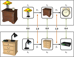
    Represents scenes as graphs that encode models and their semantic relationships, then defines a kernel between these relationship graphs that compares common virtual substructures and captures the similarity between scenes.

    paper | project page

    Matthew Fisher, Pat Hanrahan

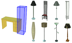
    Describe a data-driven method that uses scenes from Google 3D Warehouse to enable context-based model search of 3D scenes.

    paper | project page

    Matthew Fisher, Kayvon Fatahalian, Solomon Boulos, Kurt Akeley, Bill Mark, Pat Hanrahan

    Presents DiagSplit, a parallel algorithm for adaptively tessellating displaced parametric surfaces into high-quality, crack-free micropolygon meshes.

    paper | project page

    Matthew Fisher, Peter Schrder, Mathieu Desbrun, Hugues Hoppe

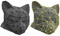
    Using tools from Discrete Exterior Calculus, we present a simple and efficient algorithm for designing tangent vector fields over arbitrary triangle meshes.

    paper | project page

    An Algorithm for the Construction of Intrinsic Delaunay Triangulations

    Matthew Fisher, Boris Springborn, Alexander Bobenko, Peter Schrder

    SIGGRAPH 2006

    Presents an algorithm for computing an intrinsic Laplace-Beltrami operator based on an intrinsic Delaunay triangulation of the surface.

    paper | project page

    This post has been generated by Page2RSS
    07 Feb 09:33

    Anatomy of Direct3D 11 Create Device

    by Chuck Walbourn - MSFT

     In answering some questions today, I remembered a topic I had been meaning to post about for some time: the seemingly simple act of creating a Direct3D 11 device. At it's core, it's pretty simple, but there's more to it than it first appears.

    The standard code for creating a Direct3D 11 device starts out pretty simple using D3D11CreateDevice:

     DWORD createDeviceFlags = 0;
    #ifdef _DEBUG
    createDeviceFlags |= D3D11_CREATE_DEVICE_DEBUG;
    #endif

    ID3D11Device* pDevice = nullptr;
    ID3D11DeviceContext* pContext = nullptr;
    D3D_FEATURE_LEVEL fl;
    HRESULT hr = D3D11CreateDevice( nullptr, D3D_DRIVER_TYPE_HARDWARE,
    nullptr, createDeviceFlags, nullptr,
    0, D3D11_SDK_VERSION, &pDevice, &fl, &pContext );

    This assumes you want the default hardware device and it handles requesting the debug device in debug builds of the application (see Direct3D SDK Debug Layer Tricks for more). This will create a device at the highest available feature level on most systems, but it has a subtle side-effect: you will never get a Feature Level 11.1 device. This is for better backwards compatibility and is easy to rectify, but for a Win32 desktop application (which can run on older versions of Windows) it's a little tricky.

    This following code is the robust way to get all possible feature levels while handling DirectX 11.0 systems:

    D3D_FEATURE_LEVEL lvl[] = { D3D_FEATURE_LEVEL_11_1, D3D_FEATURE_LEVEL_11_0,
    D3D_FEATURE_LEVEL_10_1, D3D_FEATURE_LEVEL_10_0,
    D3D_FEATURE_LEVEL_9_3, D3D_FEATURE_LEVEL_9_2, D3D_FEATURE_LEVEL_9_1 };

    DWORD createDeviceFlags = 0;
    #ifdef _DEBUG
    createDeviceFlags |= D3D11_CREATE_DEVICE_DEBUG;
    #endif

    ID3D11Device* pDevice = nullptr;
    ID3D11DeviceContext* pContext = nullptr;
    D3D_FEATURE_LEVEL fl;
    HRESULT hr = D3D11CreateDevice( nullptr, D3D_DRIVER_TYPE_HARDWARE, nullptr,
    createDeviceFlags, lvl, _countof(lvl),
    D3D11_SDK_VERSION, &pDevice, &fl, &pContext );
    if ( hr == E_INVALIDARG )
    {
    hr = D3D11CreateDevice( nullptr, D3D_DRIVER_TYPE_HARDWARE, nullptr,
    createDeviceFlags, &lvl[1], _countof(lvl)-1,
    D3D11_SDK_VERSION, &pDevice, &fl, &pContext );
    }

    The E_INVALIDARG case is the one that trips up people, and it handles the case where the platform only supports DirectX 11.0 (Windows Vista, Windows 7 RTM, or Windows 7 SP1 without KB 2670838 installed). Note you can get a similar kind of failure if you are trying to create a resource with one of the 16-bit per pixel DXGI 1.2 formats (i.e. 5/5/5/1, 565, 4/44/4) on a system with DirectX 11.0 installed.

    Direct3D 11.1

    Once you have the Direct3D device and context you can proceed, but if you want to use some of the newer features of Direct3D 11.1 you'll need another step:

     ID3D11Device1* pDevice1 = nullptr;
    ID3D11DeviceContext1* pContext1 = nullptr;
    hr = pDevice->QueryInterface( __uuidof( ID3D11Device1 ), reinterpret_cast<void**>( &pDevice1 ) );
    if ( SUCCEEDED(hr) )
    {
    (void)pContext->QueryInterface( __uuidof( ID3D11DeviceContext1 ), reinterpret_cast<void**>( &pContext1 ) );
    }

    This code requires you include <d3d11_1.h> and have the Windows 8.0 SDK or Windows 8.1 SDK. You will get a valid pDevice1 and pContext1 pointer on Windows 8.1, Windows 8.0, and Windows 7 SP1 with KB 2670838 installed.

    Direct3D 11.2

    If you want to use Direct3D 11.2 features, you do basically the same thing:

     ID3D11Device2* pDevice2 = nullptr;
    ID3D11DeviceContext2* pContext2 = nullptr;
    hr = pDevice->QueryInterface( __uuidof( ID3D11Device2 ), reinterpret_cast<void**>( &pDevice2 ) );
    if ( SUCCEEDED(hr) )
    {
    (void)pContext->QueryInterface( __uuidof( ID3D11DeviceContext2 ), reinterpret_cast<void**>( &pContext2 ) );
    }

    This code requires you include <d3d11_2.h> and have the Windows 8.1 SDK. You will get a valid pDevice2 and pContext2 pointer on Windows 8.1.

    DXGI

    The primary reason to get a DXGI interface is to enumerate adapters and inputs, but you also use them to create swap chains. There's a trick to making sure you get it robustly if you have passed 'null' to D3D11CreateDevice for the pAdapter pointer as we have above. Mixing different DXGI factory versions can cause problems, so ideally we want to use whatever the system used internally. You can do this with a little COM sequence that is perhaps familiar to Windows Store app and Xbox One developers:

     IDXGIFactory1* dxgiFactory = nullptr;
    {
    IDXGIDevice* dxgiDevice = nullptr;
    hr = pDevice->QueryInterface( __uuidof( IDXGIDevice ), reinterpret_cast<void**>( &dxgiDevice ) );
    if ( SUCCEEDED(hr) )
    {
    IDXGIAdapter* adapter = nullptr;
    hr = dxgiDevice->GetAdapter( &adapter );
    if ( SUCCEEDED(hr) )
    {
    hr = adapter->GetParent( __uuidof( IDXGIFactory1 ), reinterpret_cast<void**>( &dxgiFactory ) );
    if ( SUCCEEDED(hr) )
    {
    ...
    }
    adapter->Release();
    }
    dxgiDevice->Release();
    }
    }

    This particular sequence is a bit less verbose when using Microsoft::WRL::ComPtr.

    If you want to specify a particular adapter for the device creation, you need a DXGI factory. For DirectX 11 systems generally, you use CreateDXGIFactory1 (CreateDXGIFactory was for Direct3D 10 systems). You can make use of CreateDXGIFactory2 on Windows 8.1 systems to specify DXGI debugging, but generally you use CreateDXGIFactory1 and then would QueryInterface other versions as needed.

    Microsoft Basic Render Driver

    In the original code, we use D3D_DRIVER_TYPE_HARDWARE. If you had wanted to use the WARP software device, you would have used D3D_DRIVER_TYPE_WARP. WARP is exceptionally useful as a much faster 'ref' for testing and can be used quite successfully as a software fallback for many kinds of applications, but it is still a software renderer. As such, most games don't expect to be running under WARP.

    With Windows 8.0 and Windows 8.1, however, there is new situation to be aware of (see Desktop Games on Windows 8.x). In older versions of Windows, if a suitable video driver was not available it would fallback to a legacy VGA driver. Direct3D device creation with this driver would fail, which poses a problem for a desktop which requires it. Therefore, with Windows 8.x it defaults to the "Microsoft Basic Render Driver" instead. This is an extremely simple video output driver combined with WARP. This is a reasonable setup for servers, and the technology is very useful in making remote desktop work well.

    For games, the most likely situation for this to come up is related to the fact that Direct3D9 era hardware is considered legacy for Windows 8.x. Users can obtain older Windows Vista WDDM 1.0 or Windows 7 WDDM 1.1 drivers for their DirectX9 era video cards, but the expectation is that most x86/x64 systems will have a DirectX 10+ capable video card. Users who upgrade their systems with a DX9 video card could be running the "Microsoft Basic Render Driver" and not realize they are missing a needed driver or that their video card is too old to be supported at all (i.e. it only has an XPDM driver available which are not supported by Windows 8.x)

    One way to mitigate this scenario is for a game to detect if Microsoft Basic Render driver is active and warn the user. This is easy to do since the "Microsoft Basic Render Driver" has a well-known VendorID/DeviceID combination:

     IDXGIDevice* dxgiDevice = nullptr;
    hr = pDevice->QueryInterface( __uuidof( IDXGIDevice ), reinterpret_cast<void**>( &dxgiDevice ) );
    if ( SUCCEEDED(hr) )
    {
    IDXGIAdapter* adapter = nullptr;
    hr = dxgiDevice->GetAdapter( &adapter );
    if ( SUCCEEDED(hr) )
    {
    DXGI_ADAPTER_DESC desc;
    hr = adapter->GetDesc( &desc );
    if ( SUCCEEDED(hr) )
    {
    if ( ( desc.VendorId == 0x1414 ) && ( desc.DeviceId == 0x8c ) )
    {
    // WARNING: Microsoft Basic Render Driver is active.
    // Performance of this application may be unsatisfactory.
    // Please ensure that your video card is Direct3D10/11 capable
    // and has the appropriate driver installed.
    }
    }
    adapter->Release();
    }
    dxgiDevice->Release();
    }

    Note: If you are still supporting a Direct3D 9 game, you can detect this the same way:

     IDirect3D9* d3ddevice = Direct3DCreate9(D3D_SDK_VERSION);
    if ( d3ddevice )
    {
    D3DADAPTER_IDENTIFIER9 adapterIdentifier;
    HRESULT hr = d3ddevice->GetAdapterIdentifier(D3DADAPTER_DEFAULT, 0, &adapterIdentifier);
    if ( SUCCEEDED(hr) )
    {
    if ( ( adapterIdentifier.VendorId == 0x1414 ) && ( adapterIdentifier.DeviceId == 0x8c ) )
    {
    // WARNING: Microsoft Basic Render Driver is active.
    // Performance of this application may be unsatisfactory.br / // Please ensure that your video card is Direct3D9 capablebr / // and has the appropriate driver installed.br / }br / /code/prediv style="clear:both;"/divimg src="http://blogs.msdn.com/aggbug.aspx?PostID=10497048" width="1" height="1"
    07 Feb 09:33

    8 Visual Studio debugging tips – debug like a boss

    by Damien Guard

    There are so many useful debugging features built into Visual Studio that aren’t well known. Here are a few my favorites including some recent finds in VS 2013.

    1. Breakpoint inside a lambda

    If you click the left gutter to set breakpoints you could be easily mislead into thinking breakpoints happen at line level.

    You can actually insert a breakpoint inside parts of the line such as inside a lambda in your LINQ expression. Just right-click the part of the code and choose Breakpoint > Insert breakpoint from the context menu.

    2. Usable output window

    Visual Studio output window filtering optionsThe output window is useful for debugging where breakpoints would be too invasive or interrupt flow but it’s pretty noisy.

    Just right click in the output window (make sure output is set to debug) and turn off the Module Load, Module Unload, Process Exit and Thread Exit to leave you with stuff you actually care about. Now Debug.WriteLine to your heart’s content.

    You can also press CtrlS in the output window to save the contents.

    3. Attach debugger to client and server (VS 2012)

    It’s useful to have both server and client projects in a single solution so you only need one copy of Visual Studio running and don’t get lost alt-tabbing back and forth especially if they share common code such as a data model project.

    One disadvantage is that the start-up project is the only one to get a debugger attached. If you encounter an exception it will show in your client not your server project.

    That’s easily solved now. Right-click on the solution, choose properties and choose Multiple startup projects then select the Start action for the projects you need to attach to.

    Visual Studio Solution properties dialog

    4. Create a repro project template

    If you’re responsible for a SDK or API create a simple application that uses your stuff in a small self-contained way. Then use File > Export template… to save it.

    Now you can create a new project from your template whenever you need it with a few clicks. Even better make it available to users and testers so they can send you minimal repros.

    5. Use the DebuggerDisplay attribute

    By default the debugger will use ToString() for watch and auto windows which normally outputs class name. Even if you overwrote ToString it’s probably not what somebody debugging wants to see at a glance.

    Add DebuggerDisplay to your class with a simple expression to evaluate properties instead. e.g.:

    [DebuggerDisplay("Order {ID,nq}")
    class Order {
        public string ID { get { return id; } }
    }

    The “nq” prevents double-quotes from being emitted. You can also use methods here too but don’t do anything with subtle side-effects otherwise your observation of the subject will change its behavior and could cause weird issues.

    6. Manage breakpoints

    You set-up some interesting breakpoints and now you need to switch one off for as it’s getting hit too much but you’ll need it again in a minute. If you remove the breakpoint you’ll have to come back and find it again.

    Enter the much-overlooked Breakpoints window CtrlAltB. This will show all breakpoints you have set but crucially lets you disable them without unsetting them by simply removing the check-mark. Check it again to re-enable it.

    Visual Studio breakpoints window

    This window also provides the ability to quickly:

    • Condition when a breakpoint should occur
    • Hit count to see how often it is hit and to only break based on that count
    • Label a breakpoint to allow toggling on and off in batches
    • When Hit to put a message in the output window instead of actually breaking

    7. Break on or output the caller information (.NET 4.5/Windows 8 Store)

    There isn’t a global variable for the current method of the caller and getting the current stack can be a very slow operation.

    One quick and simple trick is to add an extra optional string parameter to the method with the CallerMemberName attribute. e.g.

    void MyFunction(string someValue, [CallerMemberName] string caller = null) {
        ...
    }

    Because it is an optional value you don’t need to modify any callers but you can now:

    1. Set a breakpoint condition inside DoSomething based on the caller variable
    2. Output the contents of caller to a log or output window

    You can also use CallerLineNumber and CallerFilePath. Also remember that constructors, finalizers and operator overloads will display their underlying method names (.ctor, op_Equals etc).

    8. See the value returned by a function (VS 2013, .NET 4.5.1/Windows 8.1 Store)

    Visual Studio autos windowSometimes you want to see what a function returned but you can’t easily because you didn’t store the value because it was the input to another function.
    This was added in VS 2013 but is incredibly easy to miss as you have to be in the right place at the right time. The right place is the Autos window and the right time is exactly the step that returned you to where the function was called from. You won’t see this before you call the function or while in the function. It’s there for a single step and looks like this:

    The arrow icon indicates it’s a return value and it lets you know the name of the function alongside it.

    Wrap up

    I also can’t stress enough how useful having logs are for troubleshooting once the software leaves your machine but that’s a much bigger discussion than this one.

    Am I missing some great debugging tips? Feel free to let me know below :)

    PS: Michael Parshin has some great tips on debugging too.

    [)amien

    07 Feb 09:32

    Porting from Windows to Linux, part 1

    by Anteru

    Hi and welcome to a blog series about how to port graphics applications from Windows to Linux. The series will have three parts: Today, in the first part, we’ll be looking at prerequisites for porting. These are things you can do any time to facilitate porting later on, while still working on Windows exclusively. In the second part, the actual porting work will be done, and in the last part, I’ll talk a bit about the finishing touches, rough edges, and how to keep everything working. All of this is based on my experience with porting my research framework; which is a medium-sized project (~ 180 kLoC) that supports Linux, Windows and Mac OS X.

    However, before we start, let’s assess the state of the project before the porting begins. For this series, I assume you have a Visual Studio based solution written in C++, with Direct3D being used for graphics. Your primary development environment is Visual Studio, and you haven’t developed for Linux before. You’re now at the point where you want to add Linux support to your application while keeping Windows intact — so we’re not talking about a rushed conversion from Windows to Linux, but of a new port of your application which will be maintained and supported alongside the Windows version.

    Prerequisites

    Let’s start by sorting out the obvious stuff: Your need a source control solution which will work on Linux. If your project is stored in TFS, now is the time to export everything to your favourite portable source control. If you are not sure what to choose, take Mercurial, which comes with a nice UI for all platforms.

    Next, check all your dependencies. If you rely on WIC for image loading, you’ll have to find a portable solution first. In my experience, it’s usually easier to have the same code running on Windows and Linux later on than having a dedicated path for each OS. In my project, I wrapped the low-level libraries like libpng or libjpg directly instead of using a larger image library.

    Now is also the time to write tests. You’ll need to be able to quickly verify that everything is working again. If you haven’t written any automated tests yet, this is the moment to start. You’ll mostly need functional tests, for instance, for disk I/O, so focus on those first. I say mostly functional tests, as unit tests tend to be OS agnostic. In my framework, unit tests cover low-level OS facilities like threads and memory allocators, while everything else, including graphics, is covered by functional tests.

    For testing, I can highly recommend Google Test. It’s not designed for functional tests right away, but it’s very easy to write a wrapper around a Google Test enabled project for functional testing. My wrapper is written in Python and sets up a new folder for each functional test, executes each test in a new process and gathers all results.

    Finally, if you have any build tools, make sure that those are portable now. I used to write them in C# when it was really new, but since a few years, I use only Python for build tools. Python code tends to be easy to maintain and it requires no build process whatsoever, making it ideally suited for build system infrastructure. Which brings us to the most important issue, the build sytem.

    Build system

    If you are using Visual Studio (or MSBuild from the command line), stop right now and start porting it to a portable build system. While in theory, MSBuild is portable to Linux using xbuild, in practice, you’ll still want to have a build system which is developed on all three platforms and used for large code bases. I have tried a bunch of them and finally settled with CMake. It uses an arcane scripting language, but it works, and it works reliably on Windows, Linux, and Mac OS X.

    Porting from Visual Studio to CMake might seem like a huge effort at first, but it’ll make the transition to Linux much easier later on. The good thing about CMake is that it works perfectly on Windows and it produces Visual Studio project files, so your existing Windows developer experience remains the same. The only difference is that adding new source files now requires you to edit a text file instead of using the IDE directly, but that’s about it.

    While writing your CMake files, here’s a few things you should double-check:

    • Are your path names case-sensitive? Windows doesn’t care, but on Linux, your include directory won’t be found if you mess up paths.
    • Are you setting compiler flags directly? Check if CMake already sets them for you before adding a huge list of compiler flags manually.
    • Are your dependencies correctly set up? With Visual Studio, it’s possible to not define all dependencies correctly and still get a correct build; while other build tools will choke on it. Use the graph output of CMake to visualize the dependencies and double check both the build order, and the individual project dependencies.

    With CMake, you should also take advantage of the “Find” mechanism for dependencies. On Linux, nearly all dependencies are available as system libraries, serviced by the package manager, so it definitely makes sense to link against the system version of a dependency if it is recent enough.

    The end result of this step should be exactly the same binaries as before, but using CMake as the build system instead of storing the solutions directly in source control. Once this is done, we can start looking at the code.

    Clean code

    Did you ever #include system headers like <windows.h> in your code? Use system types like DWORD? Now is the time to clean up and to isolate these things. You want to achieve two goals here:

    • Remove system includes from headers as much as possible.
    • Remove any Visual C++ specific code.

    System headers should be only included in source files, if possible. If not, you should isolate the classes/functions and provide generic wrappers around them. For instance, if you have a class for handling files, you can either use the PIMPL idiom or just derive a Windows-specific class from it. The second solution is usually simpler if your file class is already derived from somewhere (a generic stream interface, for instance.) Even if not, we’re wrapping an extremely slow operating system function here (file reads will typically hit the disk), so the cost of a virtual function call won’t matter in practice.

    To get rid of Visual C++ specific code, turn on all warnings and treat them as errors. There are a bunch of bogus warnings you can disable (I’ve blogged about them previously), but everything else should get fixed now. In particular, you don’t want any Visual C++ specific extensions enabled in headers. The reason why you want all warnings to be fixed is that on Linux, you’ll be getting hundreds of compile errors and warnings at first, and the less these are swamped by issues that are also present on Windows, the better.

    While cleaning up, you should pay special attention to integer sizes. Windows uses 32-bit longs in 64-bit mode, Linux defaults to 64-bit longs. To avoid any confusion, I simply use 64-bit integers when it comes to memory sizes.

    The better you clean up your code, the less work you’ll have to spend later during porting. The goal here should be to get everything to build on Windows, with platform specific files identified and isolated.

    So much for today! Next week, we’ll look at how to get rid of Direct3D and how to start bringing up the code base on Linux. Stay tuned!

    07 Feb 09:32

    PotreeConverter – sourcecode

    by mschuetz

    The PotreeConverter sourcecode can be downloaded here:
    PotreeConverter – source

    It includes a Visual Studio 2012 solution. There is no linux build but I don’t think I’ve used any platform dependend code so it shouldn’t be hard to create one.

    For anyone interested in how it works, here is a documentation. It’s written for a course I attended and explains the algorithm, not the source code.
    PotreeConverter – documentation

    07 Feb 09:30

    02-06-14 - Understanding ANS - 8

    by cbloom
    Time to address an issue that we've skirted for some time - how do you make the output string sort order?

    Recall : The output string contains Fs occurances of each symbol. For naive rANS the output string is just in alphabetical order (eg. "AAABBBCCC"). With tANS we can use any permutation of that string.

    So what permutation should we use? Well, the output string determines the C() and D() encode and decode tables. It is in fact the only degree of freedom in table construction (assuming the same constraints as last time, b=2 and L=M). So we should choose the output string to minimize code length.

    The guiding principle will be (x/P). That is, we achieve minimum total length when we make each code length as close to log2(1/P) as possible. We do that by making the input state to output state ratio (x'/x) as close to (1/P) as possible.

    (note for the record : if you try to really solve to minimize the error, it should not just be a distance between (x'/x) and (1/P) , it needs to be log-scaled to make it a "minimum rate" solution). (open question : is there an exact solution for table building that finds the minimum rate table that isn't NP (eg. not just trying all permutations)).

    Now we know that the source state always come from the precursor ranges Is, and we know that

    
    destination range :
    I = [ M , 2*M - 1]
    
    source range :
    Is = [ Fs, 2*Fs - 1 ] for each symbol s
    
    and Ps = Fs/M
    
    
    so the ideal target for the symbols in each source range is :
    
    target in I = (1/Ps) * (Is) = (M/Fs) * [ Fs, 2*Fs - 1 ] = 
    
    and taking off the +M bias to make it a string index in the range [0,M-1] :
    
    Ts = target in string = target in I - M
    
    Ts = { 0 , M * 1/Fs , M * 2/Fs) , ... }
    
    
    Essentially, we just need to take each symbol and spread its Fs occurances evenly over the output string.

    Now there's a step that I don't know how to justify without waving my hands a bit. It works slightly better if we imagine that the source x was not just an integer, but rather a bucket that covers the unit range of that integer. That is, rather that starting exactly at the value "x = Fs" you start in the range [Fs,Fs+1]. So instead of just mapping up that integer by 1/P we map up the range, and we can assign a target anywhere in that range. In the paper Duda uses a bias of 0.5 for "precise initialization" , which corresponds to assuming the x's start in the middle of their integer buckets. That is :

    
    Ts = { M * (b/Fs), M* (1+b)/Fs, M * (2+b)/Fs , ... }
    
    
    with b = 0.5 for Duda's "precise initialization". Obviously b = 0.5 makes T centered on the range [0,M] , but I see no reason why that should be preferred.

    Now assuming we have these known target locations, you can't just put all the symbols into the target slots that they want, because lots of symbols want the same spot.

    For example :

    
    M=8
    Fs={3,3,2}
    
    T_A = { 8 * 0.5/3 , 8 * 1.5 / 3 , 8 * 2.5 / 3 } = { 1 1/3 , 4 , 6 2/3 }
    T_B = T_A
    T_C = { 8 * 0.5/2 , 8 * 1.5/2 } = { 2 , 6 }
    
    
    One way to solve this problem is to start assigning slots, and when you see that one is full you just look in the neighbor slot, etc. So you might do something like :
    
    initial string is empty :
    
    string = "        "
    
    put A's in 1,4,6
    
    string = " A  A A "
    
    put B's in 1,4,6 ; oops they're taken, shift up one to find empty slots :
    
    string = " AB ABAB"
    
    put C's in 2,6 ; oops they're taken, hunt around to find empty slots :
    
    string = "CABCABAB"
    
    
    now obviously you could try to improve this kind of algorithm, but there's no point. It's greedy so it makes mistakes in the overall optimization problem (it's highly dependant on order). It can also be slow because it spends a lot of time hunting for empty slots; you'd have to write a fast slot allocator to avoid degenerate bad cases. There are other ways.

    Another thing I should note is that when doing these target slot assignments, there's no reason to prefer the most probable symbol first, or the least probable or whatever. The reason is every symbol occurance is equally probable. That is, symbol s has frequency Fs, but there are Fs slots for symbol s, so each slot has a frequency of 1. Every slot has an equal probability of 1/M.

    An alternative algorithm that I have found to work well is to sort the targets. That is :

    
    make a sorting_array of size M
    
    add { Ts, s } to sorting_array for each symbol  (that's Fs items added)
    
    sort sorting_array by target location
    
    the symbols in sorting_array are in output string order
    
    
    I believe that this is identical to Duda's "precise initialization" which he describes using push/pop operations on a heap; the result is the same - assigning slots in the order of desired target location.

    Using the sort like this is a little weird. We are no longer explicitly trying to put the symbols in their target slots. But the targets (Ts) span the range [0, M] and the sort is an array of size M, so they wind up distributed over that range. In practice it works well, and it's fast because sorting is fast.

    A few small notes :

    You want to use a "stable" sort, or bias the target by some small number based on the symbol. The reason is you will have lots of ties, and you want the ties broken consistently. eg. for "AABBCC" you want "ABCABC" or "CBACBA" but not "ABCCAB". One way to get a stable sort is to make the sorting_array work on U32's, and pack the sort rank into the top 24 bits and the symbol id into the bottom 8 bits.

    The bias = 0.5 that Duda uses is not strongly justified, so I tried some other numbers. bias = 0 is much worse. It turns out that bias = 1.0 is better. I tried a bunch of values on a large test set and found that bias = 1 is consistently good.

    One very simple way to get a decent sort is to bit-reverse the rANS indexes. That is, start from a rANS/alphabetical order string ("AABB..") and take the index of each element, bit-reverse that index (so 0001 -> 1000) , and put the symbol in the bit reversed slot. While this is not competitive with the proper sort, it is simple and one pass.

    Another possible heuristic is to just scatter the symbols by doing steps that are prime with M. This is what Yann does in fse.c

    
    All the files in Calgary Corpus :
    (compression per file; sum of output sizes)
    
    M = 1024
    
    rANS/alpahabetical : 1824053.75
    
    bit reverse : 1805230.75
    
    greedy search for empty slots : 1801351
    
    Yann's heuristic in fse.c : 1805503.13
    
    sort , bias = 0.0 : 1817269.88
    
    sort , bias = 0.5 : 1803676.38  (Duda "precise")
    
    sort , bias = 1.0 : 1798930.75


    Before anyone throws a fit - yes, I tested on my very large test set, not just calgary. The results were consistent on all the test sets I tried. I also tested with larger M (4096) and the results were again the same, though the differences are smaller the larger you make M.

    For completeness, here is what the sorts actually do :

    
    rANS/alphabetical : AAAAAAABBBBBBCCC
    
    bit reverse :   ABABABACABACABBC
    
    greedy search : CABABACABABACABB
    
    greedy search, LPS first :  ABCABAACBABACBAB
    
    Yann fse :          AAABBCAABBCAABBC
    
    sort , bias = 0.0 : ABCABABCABABCABA
    
    sort , bias = 0.5 : ABCABABACBABACBA
    
    sort , bias = 1.0 : ABABCABABCABAABC
    
    
    but I caution against judging sorts by whether they "look good" since that criteria does not seem to match coding performance.

    Finally for clarity, here's the code for the simpler sorts :

    
    void make_sort(int * sorted_syms, int sort_count, const uint32 * normalized_counts, int alphabet)
    {
        ASSERT( (int) cb::sum(normalized_counts,normalized_counts+alphabet) == sort_count );
        
        const int fse_step = (sort_count>>1) + (sort_count>>3) + 1;
        
        int fse_pos = 0;
        int s = 0;
        for LOOP(a,alphabet)
        {
            int count = normalized_counts[a];
    
            for LOOP(c,count)
            {
                // choose one :
    
                // rANS :
                sorted_syms[s] = a;
    
                // fse :
                sorted_syms[fse_pos] = a;
                fse_pos = (fse_pos + step) % sort_count;
    
                // bitreverse :
                sorted_syms[ bitreverse(s, numbits(sort_count)) ] = a;
    
                s++;
            }
        }
    }
    
    
    and the code for the actual sorting sort (recommended) :
    
    struct sort_sym
    {
        int sym;
        float rank;
        bool operator sort_sym> sort_syms;
        sort_syms.resize(sort_count);
    
        int s = 0;
    
        for LOOP(sym,alphabet)
        {
            uint32 count = normalized_counts[sym];
            if ( count == 0 ) continue;
            
            float invp = 1.f / count;
            
            float base =  1.f * invp; // 0.5f for Duda precise
    
            for LOOP(c,(int)count)
            {
                sort_syms[s].sym = sym;
                sort_syms[s].rank = base + c * invp;
                s++;
            }
        }
        
        ASSERT_RELEASE( s == sort_count );
        
        std::stable_sort(sort_syms.begin(),sort_syms.end());
        
        for LOOP(s,sort_count)
        {
            sorted_syms[s] = sort_syms[s].sym;
        }
    }
    
    
    and for the greedy search :
    
    void make_sort(int * sorted_syms, int sort_count, const uint32 * normalized_counts, int alphabet)
    {
        ASSERT( (int) cb::sum(normalized_counts,normalized_counts+alphabet) == sort_count );
    
        // make all slots empty :
        for LOOP(s,sort_count)
        {
            sorted_syms[s] = -1;
        }
        
        for LOOP(a,alphabet)
        {
            uint32 count = normalized_counts[a];
            if ( count == 0 ) continue;
            
            uint32 step = (sort_count + (count/2) ) / count;
            uint32 first = step/2;
            
            for LOOP(c,(int)count)
            {
                uint32 slot = first + step * c;
                
                // find an empty slot :
                for(;;)
                {
                    if ( sorted_syms[slot] == -1 )
                    {
                        sorted_syms[slot] = a;
                        break;
                    }
                    slot = (slot + 1)%sort_count;
                }
            }
        }
    }
    
    
    small note : the reported results use a greedy search that searches away from slot using +1,-1,+2,-2 , instead of the simpler +1,+2 in this code snippet. This simpler version is very slightly worse.

    06 Feb 07:50

    Assertions Are Pessimistic, Assumptions Are Optimistic

    by regehr

    We assert a condition when we believe it to be true in every non-buggy execution of our program, but we want to be notified if this isn’t the case. In contrast, we assume a condition when our belief in its truth is so strong that we don’t care what happens if it is ever false. In other words, while assertions are fundamentally pessimistic, assumptions are optimistic.

    C and C++ compilers have a large number of built-in assumptions. For example, they assume that every pointer that is dereferenced refers to valid storage and every signed math operation fails to overflow. In fact, they make one such assumption for each of the hundreds of undefined behaviors in the languages. Assumptions permit the compiler to generate fast code without working too hard on static analysis.

    This post explores the idea of a general-purpose assume mechanism. Although this isn’t found (as far as I know — please leave a comment if you know of something) in any commonly-used programming language, it might be useful when we require maximum performance. Although an assume mechanism seems inherently unsafe, we could use it in a safe fashion if we used a formal methods tool to prove that our assumptions hold. The role of the assumption mechanism, then, is to put high-level knowledge about program properties — whether from a human or a formal methods tool — into a form that the compiler can exploit when generating code.

    Standard C has the “restrict” type qualifier that lets the compiler assume that the pointed-to object is not aliased by other pointers. Let’s consider this (deliberately silly) function for summing up the elements of an array:

    void sum (int *array, int len, int *res)
    {
      *res = 0;
      for (int i=0; i<len; i++) {
        *res += array[i];
      }
    }
    

    The problem that the compiler faces when translating this code is that res might point into the array. Thus, *res has to be updated in every loop iteration. GCC and Clang generate much the same code:

    sum:    movl	$0, (%rdx)
            xorl	%eax, %eax
    .L2:    cmpl	%eax, %esi
    	jle	.L5
    	movl	(%rdi,%rax,4), %ecx
    	incq	%rax
    	addl	%ecx, (%rdx)
    	jmp	.L2
    .L5:    ret
    

    Both compilers are able to generate code that is five times faster — using vector instructions — if we change the definition of sum() to permit the compiler to assume that res is not an alias for any part of array:

    void sum (int *restrict array, int len, int *restrict res)
    

    Another form of assumption is the __builtin_unreachable() primitive supported by GCC and Clang, which permits the compiler to assume that a particular program point cannot be reached. In principle __builtin_unreachable() is trivial to implement: any unconditionally undefined construct will suffice:

    void unreachable_1 (void)
    {
      int x;
      x++;
    }
    
    void unreachable_2 (void)
    {
      1/0;
    }
    
    void unreachable_3 (void)
    {
      int *p = 0; 
      *p;
    }
    
    void unreachable_4 (void)
    {
      int x = INT_MAX;
      x++;
    }
    
    void unreachable_5 (void)
    {
      __builtin_unreachable ();
    }
    

    But in practice the compiler’s interpretation of undefined behavior is not sufficiently hostile — bet you never thought I’d say that! — to drive the desired optimizations. Out of the five functions above, only unreachable_5() results in no code at all being generated (not even a return instruction) when a modern version of GCC or Clang is used.

    The intended use of __builtin_unreachable() is in situations where the compiler cannot infer that code is dead, for example following a block of inline assembly that has no outgoing control flow. Similarly, if we compile this code we will get a return instruction at the bottom of the function even when x is guaranteed to be in the range 0-2.

    int foo (int x)
    {
      switch (x) {
      case 0: return bar(x);
      case 1: return baz(x);
      case 2: return buz(x);
      }
      return x; // gotta return something and x is already in a register...
    }
    

    If we add a __builtin_unreachable() at the bottom of the function, or in the default part of the switch, then the compiler drops the return instruction. If the assumption is violated, for example by calling foo(7), execution will fall into whatever code happens to be next — undefined behavior at its finest.

    But what about the general-purpose assume()? This turns out to be easy to implement:

    void assume (int expr)
    {
      if (!expr) __builtin_unreachable();
    }
    

    So assume() is using __builtin_unreachable() to kill off the collection of program paths in which expr fails to be true. The interesting question is: Can our compilers make use of assumptions to generate better code? The results are a bit of a mixed bag. The role of assume() is to generate dataflow facts and, unfortunately, the current crop of compilers can only be trusted to learn very basic kinds of assumptions. Let’s look at some examples.

    First, we might find it annoying that integer division in C by a power of 2 cannot be implemented using a single shift instruction. For example, this code:

    int div32 (int x)
    {
      return x/32;
    }
    

    Results in this assembly from GCC:

    div32:  leal	31(%rdi), %eax
    	testl	%edi, %edi
    	cmovns	%edi, %eax
    	sarl	$5, %eax
    	ret
    

    And this from Clang:

    div32:  movl	%edi, %eax
    	sarl	$31, %eax
    	shrl	$27, %eax
    	addl	%edi, %eax
    	sarl	$5, %eax
    	ret
    

    The possibility of a negative dividend is causing the ugly code. Assuming that we know that the argument will be non-negative, we try to fix the problem like this:

    int div32_nonneg (int x)
    {
      assume (x >= 0);
      return div32 (x);
    }
    

    Now GCC nails it:

    div32_nonneg:
    	movl	%edi, %eax
    	sarl	$5, %eax
    	ret
    

    Clang, unfortunately, generates the same code from div32_nonneg() as it does from div32(). Perhaps it lacks the proper value range analysis. I’m using Clang 3.4 and GCC 4.8.2 for this work, by the way. UPDATE: In a comment Chris Lattner provides a link to this known issue in LLVM.

    Next we’re going to increment the value of each element of an array:

    void inc_array (int *x, int len)
    {
      int i;
      for (i=0; i<len; i++) {
        x[i]++;
      }
    }
    

    The code generated by GCC -O2 is not too bad:

    inc_array:
    	testl	%esi, %esi
    	jle	.L18
    	subl	$1, %esi
    	leaq	4(%rdi,%rsi,4), %rax
    .L21:   addl	$1, (%rdi)
    	addq	$4, %rdi
    	cmpq	%rax, %rdi
    	jne	.L21
    .L18:   rep ret
    

    However, is that test at the beginning really necessary? Aren’t we always going to be incrementing an array of length at least one? If so, let’s try this:

    void inc_nonzero_array (int *x, int len)
    {
      assume (len > 0);
      inc_array (x, len);
    }
    

    Now the output is cleaner:

    inc_nonzero_array:
    	subl	$1, %esi
    	leaq	4(%rdi,%rsi,4), %rax
    .L24:   addl	$1, (%rdi)
    	addq	$4, %rdi
    	cmpq	%rax, %rdi
    	jne	.L24
    	rep ret
    

    The preceding example was suggested by Arthur O’Dwyer in a comment on my assertion post.

    If you readers have any good examples where non-trivial assumptions result in improved code, I’d be interested to see them.

    Next, let’s look at the effect of assumptions in a larger setting. I compiled LLVM/Clang in four different modes. First, in its default “Release+Assertions” configuration. Second, in a “minimal assert” configuration where assert() was defined like this:

    #define assert(expr) ((expr) ? static_cast<void>(0) : _Exit(-1))
    

    This simply throws away the verbose failure information. Third, in a “no assert” configuration where assert() was defined like this:

    #define assert(expr) (static_cast<void>(0))
    

    Fourth, I turned each assertion in LLVM/Clang into an assumption like this:

    #define assert(expr) ((expr) ? static_cast<void>(0) : __builtin_unreachable())
    

    Then I built each of the configurations using GCC 4.8.2 and Clang 3.4, giving a total of eight Clang binaries as a result. Here’s the code size:

    Bear in mind that the y-axis doesn’t start at zero, I wanted to make the differences stand out. As expected, default assertions have a heavy code size penalty. Perhaps interestingly, GCC was able to exploit assumptions to the point where there was a small overall code size win. LLVM did not manage to profit from assumptions. Why would assumptions have a code size penalty over no assertions? My guess is that some assumptions end up making function calls that cannot be optimized away, despite their lack of side effects.

    Now let’s look at the performance of the eight clangs. The benchmark here was optimized compilation of a collection of C++ files. Each number in the graph is the median value of 11 reps, but really this precaution was not necessary since there was very little variance between reps. Note again that the y-axis doesn’t start at zero.

    Both compilers are slowed down by assumes. Again, I would guess this is because sometimes the compiler cannot elide function calls that are made during the computation of a expression that is being assumed.

    One surprise from these graphs is that Clang is generating code that is both smaller and faster than GCC’s. My view (formed several years ago) has been that Clang usually produces slightly slower code, but requires less compile time to do it. This view could easily have become invalidated by rapid progress in the compiler. On the other hand, since the code being compiled is LLVM/Clang itself, perhaps we should expect that Clang has been extensively tuned to generate good object code in this case.

    A not-surprise from these graphs is that we generally cannot just take a big collection of assertions, turn them into assumptions, and expect good results. Getting good results has two parts: an easy one and a hard one. The easy part is selectively removing assumptions that are hurting more than they help. These would tend to be complex conditions that are slow to compute and that have no chance of generating dataflow facts that the compiler can make use of. This picking and choosing could even be done automatically.

    The second part of getting good results out of assumptions is creating compilers that are more generally capable of learning and exploiting arbitrary new dataflow facts provided by users. In the short run, this is a matter of testing and fixing and tuning things up. In the long run, my belief is that compilers are unnecessarily hampered by performance constraints — they have to be pretty fast, even when compiling large codes. An alternative is to support a “-Osearch” mode where the compiler spends perhaps a lot of time looking for better code sequences; see this comment from bcs. The compiler’s search could be randomized or it could involve integration with an SMT solver. Companies that burn a lot of CPU cycles in server farms should be highly motivated to optimize, for example, the 500 functions that use the most power every day. I’m assuming that some sort of systematic cluster-wide profiling facility exists, we don’t want to waste time optimizing code unless it’s causing pain.

    The postcondition of any assumption is the same as the postcondition of asserting the same expression. Thus, we can see that asserts can also make our code faster — but this requires the speedup from the extra dataflow facts to outweigh the slowdown from the assertion check. I don’t know that anyone has ever looked into the issue of when and where assertions lead to faster code. We would not expect this to happen too often, but it would be cute if compiling some big program with -DNDEBUG made it slower.

    Although they would normally be used to support optimization, I believe that assumptions can also directly support bug detection. A tool such as Stack could be modified to analyze a program with the goal of finding code that becomes dead due to an assumption. The presence of such code is likely to signal a bug.

    In summary, assume() is a mechanism for introducing new undefined behaviors into programs that we write. Although this mechanism would be easy to misuse, there’s no reason why it cannot be used safely and effectively when backed up by good programming practices and formal methods.

    06 Feb 07:48

    02-05-14 - Understanding ANS - 7

    by cbloom
    And we're ready to cover table-based ANS (or "tANS") now.

    I'm going to be quite concrete and consider a specific choice of implementation, rather than leaving everything variable. But extrapolation to the general solution is straightforward.

    You have integer symbol frequences Fs. They sum to M. The cumulative frequencies are Bs.

    I will stream the state x in bits. I will use the smallest possible renormalization range for this example , I = [ M , 2*M - 1]. You can always use any integer multiple of M that you want (k*M, any k), which will give you more coding resolution (closer to entropy). This is equivalent to scaling up all the F's by a constant factor, so it doesn't change the construction here.

    Okay. We will encode/decode symbols using this procedure :

    
    ENCODE                      DECODE
    
    |                           ^
    V                           |
    
    stream out                  stream in
    
    |                           ^
    V                           |
    
    C(s,x) coding function      D(x) decoding function
    
    |                           ^
    V                           |
    
    x'                          x'
    
    
    We need tables for C() and D(). The constraints are :
    
    D(x') = { x , s }  outputs a state and a symbol
    
    D(x) must be given for x in I = [ M , 2*M - 1 ]
    
    D(x) in I must output each symbol s Fs times
    
    that is, D(x in I) must be an output string made from a permutation of "AA..BB.." , each symbol Fs times
    
    D( C( s, x ) ) = { x , s }  decode must invert coding
    
    C(s,x) = x'  outputs the following state
    
    C(s,x) must be given for x' in I
     that's x in Is
    
    The precursor ranges Is = { x : C(s,x) is in I }
    must exist and be of the form Is = [ k , 2k-1 ] for some k
    
    
    Now, if we combine the precursor range requirement and the invertability we can see :
    
    D(x in I) outputs each s Fs times
    
    C(s,x) with x' in I must input each s Fs times
    
    the size of Is must be Fs
    
    the precursor ranges must be Is = [ Fs, 2*Fs - 1 ]
    
    C(s,x) must given in M slots
    
    
    And I believe that's it; those are the necessary and sufficient conditions to make a valid tANS system. I'll go over some more points and fill in some details.

    Here's an example of the constraint for an alphabet of "ABC" and M = 8 :

    Now, what do you put in the shaded area? You just fill in the output states from 8-15. The order you fill them in corresponds to the output string. In this case the output string must be some permutation of "AAABBBCC".

    Here's one way : (and in true Duda style I have confusingly used different notation in the image, since I drew this a long time ago before I started this blog series. yay!)

    In the image above I have also given the corresponding output string and the decode table. If you're following along in Duda's paper arxiv 1311.2540v2 this is figure 9 on page 18. What you see in figure 9 is a decode table. The "step" part of figure 9 is showing one method of making the sort string. The shaded bars on the right are showing various permutations of an output string, with a shading for each symbol.

    Before I understood ANS I was trying tables like this :

    
    M=16
    Fs = {7,6,3}
    
     S |  0|  1|  2
    ---|---|---|---
      1|  2|  3|  4
      2|  5|  6| 10
      3|  7|  8| 15
      4|  9| 11| 20
      5| 12| 13| 26
      6| 14| 16| 31
      7| 17| 19|   
      8| 18| 22|   
      9| 21| 24|   
     10| 23| 27|   
     11| 25| 29|   
     12| 28|   |   
     13| 30|   |   
    
    
    This table does not work. If you're in state x = 7 and you want to encode symbol 2, you need to stream out bits to get into the precursor range I2. So you stream out from x=7 and get to x=3. Now you look in the table and you are going to state 15 - that's not in the range I=[16,31]. No good!

    A correct table for those frequencies is :

    
     S |  0|  1|  2
    ---|---|---|---
      3|   |   | 18
      4|   |   | 24
      5|   |   | 29
      6|   | 17|   
      7| 16| 20|   
      8| 19| 22|   
      9| 21| 25|   
     10| 23| 27|   
     11| 26| 31|   
     12| 28|   |   
     13| 30|   |   
    
    
    Building the decode table from the encode table is trivial.

    Note that the decode table D(x) only has to be defined for x in I - that's M entries.

    C(x,s) also only has M entries. If you made it naively as a 2d array, it would be |alphabet|*M . eg. something like (256*4096) slots, but most of it would be empty. Of course you don't want to do that.

    The key observation is that C(x,s) is only defined over consecutive ranges of x for each s. In fact it's defined over [Fs, 2*Fs-1]. So, we can just pack these ranges together. The starting point in the packed array is just Bs - the cumulative frequency of each symbol. That is :

    
    PC = packed coding table
    PC has M entries
    
    C(x,s) = PC[ Bs + (x - Fs) ]
    
    
    eg. for the {3,3,2} table shown in the image above :
    
    PC = { 8,11,14, 9,12,15, 10,13 }
    
    
    this allows you to store the coding table also in an array of size M.

    There are a few topics on tANS left to cover but I'll leave them for the next post.

    06 Feb 07:45

    Comparing Filesystem Performance in Virtual Machines

    Comparing Filesystem Performance in Virtual Machines:

    In the previous post I’ve linked to, How not to benchmark Cassandra, Jonathan Ellis writes on the subject of testing on virtual machines:

    This one is actually defensible: if you deploy on VMs, then benchmarking on VMs is the most relevant scenario for you. So as long as you understand the performance hit you’re taking, this can be a reasonable choice. However, care must be taken: noisy neighbors can skew results, especially when using smaller instance sizes. Even with larger instances, it’s much more difficult than you think to get consistent results.

    This reminded me of a blog post, I’ve read earlier this year, authored by Mitchell Hashimoto in which he compares the performance of filesystems in VirtualBox and VMware with different settings:

    For years, the primary bottleneck for virtual machine based development environments with Vagrant has been filesystem performance. CPU differences are minimal and barely noticeable, and RAM only becomes an issue when many virtual machines are active. I spent the better part of yesterday benchmarking and analyzing common filesystem mechanisms, and now share those results here with you.

    Original title and link: Comparing Filesystem Performance in Virtual Machines (NoSQL database©myNoSQL)

    05 Feb 16:11

    FSE : Defining optimal subranges

    by Yann Collet
    Note : Charles Bloom started an independent in-depth analysis of ANS on his blog, which is definitely worth the read.

     As stated in earlier FSE comparison with Arithmetic Coding, FSE deals with fractional bits by "decreasing" its state value. Now how does that work precisely ?

    Let's use again the example of a symbol which probability of appearance is 5/4096. The Shannon limit for this symbol is 9.68 bits per symbol (if we do better, then some other symbols will suffer, and the overall will compress less). As stated earlier, we deal with the fractional bit issue by outputting sometimes 9 bits, sometimes 10 bits.

    The distribution of 9-bits & 10-bits sub-ranges must ensure that all possible values remain accessible after the current symbol. It's a condition for lossless compression. The result is the following layout :


    OK, so why are the 9-bits subranges positioned at the beginning of the range ?
    Well, in previous article, we said that an additional bit is read when the state is so much decreased that is goes below lower limit. In which case, it just "wraps around", starting again from the top value, at the cost of an additional bit read.


    So it's not so much that the 9-bits are at the bottom. Rather, with above explanation, it is more intuitive to explain that the 10-bits are at the top.
    Maybe it would be easier to notice with another example, a symbol with 7/4096 probability of appearance.


    Note that these subranges are "destination ranges". Each of the 7 symbol_cells are mapped to one and only one of these ranges.

    So which symbol is associated with each range ?

    As stated earlier, since the additional bit is "paid for" when crossing the low limit, the most likely symbol to trigger the limit is lowest one.
    So we give an index to each of the 7 symbol_cells, in their order of appearance, from the smaller to the larger one.
    The largest 10-bits range is attributed to symbol_cells n°1.
    The other ranges simply follow, in their natural order :


    This is coherent with an optimal cost associated with a 7/4096 distribution : 9.19 bits.
    It means that we are only consuming 0.19 fractional bits each time the symbol is decoded. So we can decode it about 5 times at 9-bits before requiring 10-bits.

    This is in contrast with a probability of 5/4096 :


    Here, the optimal cost is 9.68 bits, so fractional bits is much higher (0.68 bits). We are likely to cross the low limit much more often. Hence the first 3 symbol_cells trigger the additional bit read, and require 10 bits.

    This rule is valid for any probability; so now, whether it is 5/4096, 134/4096, or even 3812/4096, you know how to define destination sub-ranges, and can build the associated decoding table.
    (The latest example is interesting, since some sub-ranges will be 0-bits large, which means they map directly to another state value : 3812/4096 => 284 1-bit sub-ranges + 3528 0-bit sub-ranges).

    What remains to be understood is how to distribute the symbol states. A naive approach would be to simply cluster them together. For example, a symbol with probability of 7/4096 would occupy state values from 0 to 6. It would work, but compression effectiveness would be very poor.
    In another blog post, we'll see why, and how to correct that.


    05 Feb 07:07

    02-04-14 - Understanding ANS - 6

    by cbloom
    Okay, let's get to streaming.

    For illustration let's go back to the simple example of packing arbitrary base numbers into an integer :

    
    // encode : put val into state
    void encode(int & state, int val, int mod)
    {
        ASSERT( val >= 0 && val 
    as you encode, state grows, and eventually gets too big to fit in an integer. So we need to flush out some bits (or bytes).

    But we can't just stream out bits. The problem is that the decoder does a modulo to get the next value. If we stream in and out high bits, that's equivalent to doing something like +65536 on the value. When you do a mod-3 (or whatever) on that, you have changed what you decode.

    If you only ever did mod-pow2's, you could stream bits out of the top at any time, because the decoding of the low bits is not affected by the high bits. This is how the Huffman special case of ANS works. With Huffman coding you can stream in and out any bits that are above the current symbol, because they don't affect the mask at the bottom.

    In general we want to stream bits (base 2) or bytes (base 256). To do ANS in general we need to mod and multiply by arbitrary values that are not factors of 2 or 256.

    To ensure that we get decodability, we have to stream such that the decoder sees the exact value that the encoder made. That is :

    
    ENCODE                      DECODE
    
    |                           ^
    V                           |
    
    stream out                  stream in
    
    |                           ^
    V                           |
    
    C(s,x) coding function      D(x) decoding function
    
    |                           ^
    V                           |
    
    x'                          x'
    
    
    The key thing is that the value of x' that C(s,x) makes is exactly the same that goes into D(x).

    This is different from Huffman, as noted above. It's also different than arithmetic coding, which can have an encoder and decoder that are out of sync. An arithmetic decoder only uses the top bits, so you can have more or less of the rest of the stream in the low bits. While the basic ANS step (x/P + C) is a kind of arithmetic coding step, the funny trick we did to take some bits of x and mod it back down to the low bits (see earlier posts) means that ANS is *not* making a continuous arithmetic stream for the whole message that you can jump into anywhere.

    Now it's possible there are multiple streaming methods that work. For example with M = a power of 2 in rANS you might be able to stream high bytes. I'm not sure, and I'm not going to talk about that in general. I'm just going to talk about one method of streaming that does work, which Duda describes.

    To ensure that our encode & decode streaming produce the same value of x', we need a range to keep it in. If you're streaming in base b, this range is of the form [L, b*L-1] . So, I'll use Duda's terminology and call "I" the range we want x' to be in for decoding, that is

    
    I = [L, b*L-1]
    
    Decoder streams into x :
    
    x 
    but the encoder must do something a bit funny :
    
    stream out from x
    
    x' = C(s,x)  , coding function
    
    x' now in I
    
    
    that is, the stream out must be done before the coding function, and you must wind up in the streaming range after the coding function. x' in the range I ensures that the encoder and decoder see exactly the same value (because any more streaming ops would take it out of I).

    To do this, we must know the "precursor" ranges for C(). That is :

    
    Is = { x : C(s,x) is in I }
    
    that is, the values of x such that after coding with x' = C(s,x), x' is in I
    
    
    these precursor ranges depend on s. So the encoder streaming is :
    
    I'm about to encode symbol s
    
    stream out bits from x :
    
    put_base_b( x % b )
    x 
    so we get into the precursor range, and then after the coding step we are in I.

    Now this is actually a constraint on the coding function C (because it determines what the Is are). You must be able to encode any symbol from any state. That means you must be able to reach the Is precursor range for any symbol from any x in the output range I. For that to be true, the Is must span a power of b, just like "I" does. That is,

    
    all Is must be of the form
    
    Is = [ K, b*K - 1 ]
    
    for some K


    eg. to be concrete, if b = 2, we're streaming out bits, then Is = { 3,4,5 } is okay, you will be able to get there from any larger x by streaming out bits, but Is = {4,5,6} is not okay.

    
    I = [8, 15]
    
    Is = {4,5,6}
    
    x = 14
    
    x is out of Is, so stream out a bit ; 14 -> 7
    
    x is out of Is, so stream out a bit ; 7 -> 3
    
    x is below Is!  crap!
    
    
    this constraint will be our primary guide in building the table-based version of ANS.

    05 Feb 07:06

    IISPH-FLIP for Incompressible Fluids

    by christopherbatty

    J. Cornelis, M. Ihmsen, A. Peer, M. Teschner

    We propose to use Implicit Incompressible Smoothed Particle Hydrodynamics (IISPH) for pressure projection and boundary handling in Fluid-Implicit-Particle (FLIP) solvers for the simulation of incompressible fluids. This novel combination addresses two issues of existing SPH and FLIP solvers, namely mass preservation in FLIP and efficiency and memory consumption in SPH. First, the SPH component enables the simulation of incompressible fluids with perfect mass preservation. Second, the FLIP component efficiently enriches the SPH component with detail that is comparable to a standard SPH simulation with the same number of particles, while improving the performance by a factor of 7 and significantly reducing the memory consumption. We demonstrate that the proposed IISPH-FLIP solver can simulate incompressible fluids with a quantifiable, imperceptible density deviation
    below 0:1%. We show large-scale scenarios with up to 160 million particles that have been processed on a single desktop PC using only 15GB of memory. One- and two-way coupled solids are illustrated.

    IISPH-FLIP for Incompressible Fluids

    05 Feb 07:03

    Clang 3.4 and C++14

    by Scott Prager
    With each new release, gcc and clang add on more C++11 and C++14 features. While clang has been behind on some features, though ahead on others, they now claim to have C++1y all worked out.

    This article is not comprehensive.
    Clang's 3.4 C++ release notes:  http://llvm.org/releases/3.4/tools/clang/docs/ReleaseNotes.html#id1
    libc++'s C++1y status: http://libcxx.llvm.org/cxx1y_status.html

    Note: To compile these examples requires the flags, "-stdlib=libc++" and "-std=c++1y".


    Variable templates.


    This feature, from N3651, took me most be surprise, but it also seems quite obvious. In the simplest example, let def<T> be a variable that represents the default-constructed value of any type, T.

    template<typename T>
    constexpr T def = T();
     
    auto x = def<int>; // x = int()
    auto y = def<char>; // y = char() 

    The proposal uses the example of pi, where it may be more useful to store it as a float or double, or even long double. By defining it as a template, one can have precision when needed and faster, but less precise, operations otherwise.

    For another example, consider storing a few prime numbers, but not specifying the type of their container.

    template<template<typename...> class Seq>
    Seq<int> primes = { 1, 2, 3, 5, 7, 11, 13, 17, 19 };
    
    auto vec = primes<std::vector>;
    auto list = primes<std::list>;
    (gist)

    Also, the standard library contains many template meta-functions, some with a static value member. Variable templates help there, too.

    template<typename T, typename U>
    constexpr bool is_same = std::is_same<T,U>::value;
    
    bool t = is_same<int,int>;   // true
    bool f = is_same<int,float>; // false
    (std::is_same)

    But since variable templates can be specialized just like template functions, it makes as much sense to define it this way:

    template<typename T, typename U>
    constexpr bool is_same = false;
    
    template<typename T>
    constexpr bool is_same<T,T> = true;
    (gist)

    Except for when one requires that is_same refers to an integral_constant.

    One thing worries me about this feature: How do we tell the difference between template meta-functions, template functions, template function objects, and variable templates? What naming conventions will be invented? Consider the above definition of is_same and the fallowing:

    // A template lambda that looks like a template function.
    template<typename T>
    auto f = [](T t){ ... };
    
    // A template meta-function that might be better as a variable template.
    template<typename T>
    struct Func : { using value = ...; };

    They each has subtly different syntaxes. For example, N3545 adds an operator() overload to std::integral_constant which enables syntax like this: bool b = std::is_same<T,U>(), while N3655 adds std::is_same_t<T,U> as a synonym for std::is_same<T,U>::value. (Note: libc++ is missing std::is_same_t.) Even without variable templates, we have now three ways to refer to the same thing.

    Finally, one problem I did have with it is I wrote a function like so:

    template<typename T>
    auto area( T r ) {
        return pi<T> * r * r;
    };

    and found that clang thought pi<T> was undefined at link time and clang's diagnostics did little to point that out.

    /tmp/main-3487e1.o: In function `auto $_1::operator()<Circle<double> >(Circle<double>) const':
    main.cpp:(.text+0x5e3d): undefined reference to `_ZL2piIdE'
    clang: error: linker command failed with exit code 1 (use -v to see invocation

    I solved this by explicitly instantiating pi for the types I needed by adding this to main:

    pi<float>;
    pi<double>;
    

    Why in main and not in global scope? When I tried it right below the definition of pi, clang thought I wanted to specialize the type. Finally, attempting template<> pi<float>; left the value uninitialized. This is a bug in clang, and has been fixed. Until the next release, variable templates work as long as only non-template functions refer to them.


    Generic lambdas and generalized capture.


    Hey, didn't I already do an article about this? Well, that one covers Faisal Vali's fork of clang based off of the N3418, which has many more features than this iteration based off the more conservative N3559. Unfortunately it lacks the terseness and explicit template syntax (i.e. []<class T>(T t) f(t)), but it maintains automatic types for parameters ([](auto t){return f(t);}).

    Defining lambdas as variable templates helps, but variable templates lack the abilities of functions, like implicit template parameters. For the situations where that may be helpful, it's there.

    template<typename T>
    auto convert = [](const auto& x) {
        return T(x);
    };
    (gist)

    Also, previously, clang couldn't capture values by move or forward into lambdas, which prohibited capturing move-only types by anything other than a reference. Transitively, that meant many perfect forwarding functions couldn't return lambdas.

    Now, initialization is "general", to some degree.

    std::unique_ptr<int> p = std::make_unique<int>(5);
    auto add_p = [p=std::move(p)](int x){ return x + *p; };
    std::cout << "5 + 5 = " << add_p(5) << std::endl;
    
    (See also: std::make_unique)

    Values can also be copied into a lambda using this syntax, but check out Scott Meyer's article for why [x] or [=] does not mean the same thing as [x=x] for mutable lambdas. (http://scottmeyers.blogspot.de/2014/02/capture-quirk-in-c14.html)

    Values can also be defined and initialized in the capture expression.

    std::vector<int> nums{ 5, 6, 7, 2, 9, 1 };
     
    auto count = [i=0]( auto seq ) mutable {
        for( const auto& e : seq )
            i++; // Would error without "mutable".
        return i;
    };
    

    gcc has had at least partial support for this since 4.5, but should fully support it in 4.9.


    Auto function return types.


    This is also a feature gcc has had since 4.8 (and I wrote about, as well), but that was based off of N3386, whereas gcc 4.9 and clang 3.4 base off of N3638. I will not say much here because this is not an entirely new feature, not much has changed, and it's easy to groc.

    Most notably, the syntax, decltype(auto), has been added to overcome some of the shortcomings of auto. For example, if we try to write a function that returns a reference with auto, a value is returned. But if we write it...

    decltype(auto) ref(int& x) {
        return x;
    }
    
    decltype(auto) copy(int x) {
        return x;
    } 
    (gist)

    Then a reference is returned when a is given, and a copy when a value is given. (Alternatively, the return type of ref could be auto&.)


    More generalized constexprs.


    The requirement that constexprs be single return statements worked well enough, but simple functions that required more than one line could not be constexpr. It sometimes forced inefficient implementations in order to have at least some of its results generated at compile-time, but not always all. The factorial function serves as a good example.

    constexpr unsigned long long fact( unsigned long long x ) {
        return x <= 1 ? 1ull : x * fact(x-1);
    }

    but now we can write...

    constexpr auto fact2( unsigned long long x ) {
        auto product = x;
        while( --x ) // Branching.
            product *= x; // Variable mutation.
        return product;
    }
    (gist)

    This version may be more efficient, both at compile time and run time.

    The accompanying release of libc++ now labels many standard functions as constexpr thanks to N3469 (chrono), 3470 (containers), 3471 (utility), 3302 (std::complex), and 3789 (functional).

    Note: gcc 4.9 does not yet implement branching and mutation in constexprs, but does include some of the library enhancements.


    std::integer_sequence for working with tuples.


    Although this library addition may not be of use to everyone, anyone who has attempted to unpack a tuple into a function (like this guy or that guy or this one or ...) will appreciate N3658 for "compile-time integer sequences". Thus far, no standard solution has existed. N3658 adds one template class, std::integer_sequence<T,t0,t1,...,tn>, and std::index_sequence<t0,...,tn>, which is an integer_sequence with T=size_t. This lets us write an apply_tuple function like so:


    template<typename F, typename Tup, size_t ...I>
    auto apply_tuple( F&& f, Tup&& t, std::index_sequence<I...> ) {
        return std::forward<F>(f) (
             std::get<I>( std::forward<Tup>(t) )... 
        );
    }
    
    (See also: std::get)

    For those who have not seen a function like this, the point of this function is just to capture the indexes from the index_sequence and call std::get variadically. It requires another function to create the index_sequence.

    N3658 also supplies std::make_integer_sequence<T,N>, which expands to std::integer_sequence<T,0,1,...,N-1>, std::make_index_sequence<N>, and std::index_sequence_for<T...>, which expands to std::make_index_sequence<sizeof...(T)>.


    // The auto return type especially helps here.
    template<typename F, typename Tup >
    auto apply_tuple( F&& f, Tup&& t ) {
        using T = std::decay_t<Tup>; // Thanks, N3655, for decay_t.
    
        constexpr auto size = std::tuple_size<T>(); // N3545 for the use of operator().
        using indicies = std::make_index_sequence<size>; 
    
        return apply_tuple( std::forward<F>(f), std::forward<Tup>(t), indicies() ); 
    }
    
    (See also: std::decay, std::tuple_size, gist

    Unfortunately, even though the proposal uses a similar function as an example, there still exists no standard apply_tuple function, nor a standard way to extract an index_sequence from a tuple. Still, there may exist several conventions for applying tuples. For example, the function may be the first element or an outside component. The tuple may have an incomplete argument set and require additional arguments for apply_tuple to work.

    Update: Two library proposals in the works address this issue: N3802 (apply), and N3416 (language extension: parameter packs).


    experimental::optional.


    While not accepted into C++14, libc++ has an implementation of N3672's optional hidden away in the experimental folder. Boost fans may think of it as the standard's answer to boost::optional as functional programers may think of it as like Haskell's Maybe.

    Basically, some operations may not have a value to return. For example, a square root cannot be taken from a negative number, so one might want to write a "safe" square root function that returned a value only when x>0.


    #include <experimental/optional>
    
    template<typename T>
    using optional = std::experimental::optional<T>;
    
    optional<float> square_root( float x ) {
        return x > 0 ? std::sqrt(x) : optional<float>();
    }
    
    (gist)

    Using an optional is simple because they implicitly convert to bools and act like a pointer, but with value semantics (which is incidentally how libc++ implements it). Without optional, one might use a unique_ptr, but value semantics on initialization and assignment make optional more convenient.


    auto qroot( float a, float b, float c ) 
        -> optional< std::tuple<float,float> >
    {
        // Optionals implicitly convert to bools.
        if( auto root = square_root(b*b - 4*a*c) ) {
            float x1 = -b + *root / (2*a);
            float x2 = -b - *root / (2*a);
            return {{ x1, x2 }}; // Like optional{tuple{}}.
        }
        return {}; // An empty optional.
    }  
    (gist)


    Misc. improvements.


    This version of libc++ allows one to retrieve a tuple's elements by type using std::get<T>.


    std::tuple<int,char> t1{1,'a'};
    std::tuple<int,int>  t2{1,2}; 
    int x = std::get<int>(t1); // Fine.
    int y = std::get<int>(t2); // Error, t2 contains two ints.


    Clang now allows the use of single-quotes (') to separate digits. 1'000'000 becomes 1000000, and 1'0'0 becomes 100. (example) (It doesn't require that the separations make sense, but one cannot write 1''0 or '10.)

    libc++ implements N3655, which adds several template aliases in the form of std::*_t = std::*::type to <type_traits>, such as std::result_of_t, std::is_integral_t, and many more. Unfortunately, while N3655 also adds std::is_same_t (see the top of the 7th page), libc++ does not define it. I do not know, but I believe this may be an oversight that will be fixed soon as it requires only one line.

    N3421 adds specializations to the members of <functional>. If one wanted to send an addition function into another functions, one might write f(std::plus<int>(),args...), but we new longer need to specify the type and can instead write std::plus<>(). This instantiates a function object that can accept two values of any type to add them. Similarly, std::greater<>, std::less<>, std::equal_to<>, etc...


    Conclusions.


    This may not be the most ground-breaking release, but C++14 expands on the concepts from C++11, improves the library, and adds a few missing features, and I find it impressive that the clang team has achieved this so preemptively. I selected to talk about the features I thought were most interesting, but I did not talk about, for example, sized deallocation, std::dynarray (<experimental/dynarry>), some additional overloads in <algorithm>, or Null Forward Iterators, to name a few. See the bottom for links to the full lists.

    The GNU team still needs to do more work to catch up to clang. If one wanted to write code for both gcc 4.9 and clang 3.4, they could use generic lambdas, auto for return types, but not variable templates or generalized constexprs. For the library, gcc 4.9 includes std::make_unique (as did 4.8), the N3412 specializations in <functional>, integer sequences, constexpr library improvements, even experimental::optional (though I'm not sure where), and much more. It may be worth noting it does not seem to include the <type_traits> template aliases, like result_of_t.

    See clang's full release notes related to C++14 here: http://llvm.org/releases/3.4/tools/clang/docs/ReleaseNotes.html#id1
    For libc++'s improvements, see: http://libcxx.llvm.org/cxx1y_status.html
    gcc 4.9's C++14 features: http://gcc.gnu.org/projects/cxx1y.html
    And gcc's libstdc++ improvements:  http://gcc.gnu.org/onlinedocs/libstdc++/manual/status.html#status.iso.2014

    The code I wrote to test these features: https://gist.github.com/splinterofchaos/8810949