Andrew McNamara
Shared posts
Andrew Dunstan: Yet Another JSON parser for PostgreSQL
The Colors of Racism
Recently, somewhat by accident, I stumbled into reading a couple of monstrously racist texts, and I’m going to need to update the Wikipedia entry for a famous British author. But I learned a few things along the way that I want to share.
Disclosure
I try to be antiracist, but I don’t think I’m particularly good at it. I sometimes have bigoted feelings but try hard to recognize and not act on them. I’m convinced that humans are naturally tribal and antiracist work will continue to be required for the foreseeable future.
The Author
Anthony Trollope (1815-1882) wrote 47 novels. I generally like them and we own a whole shelf-full. They are funny and tender and cynical; his characters love and marry and go into business and get elected to Parliament and are corrupt and engage in furious professional conflict. Those characters are, without exception, “gentle”, by which I mean members of the British ruling class.
Anthony Trollope in 1864.
When I was traveling around the world a lot, regularly crossing major oceans before the era of in-air Internet, Trollope was a regular companion; his books tend to be big and thick and extremely readable. Want to get started? Barchester Towers, about a bitter feud among the clergymen of an English country town, is one of the funniest books ever written; also there’s an excellent BBC adaptation, with Alan Rickman deliciously smarmy as the horrid Mr Slope.
What happened was…
I’m on a publishing-oriented mailing list and someone wrote “I stumbled on the fact that Trollope wrote a book that describes race relations in the British West Indies” and someone wrote back “It’s a travelogue not a novel, it’s called The West Indies and the Spanish Main, and be careful, that race-relations stuff may not be pleasant to read.” On a whim, I summoned up the book from our excellent public-library system and, oh my goodness gracious, that “not pleasant” was understating it.
The book
Trollope earned his living, while he was establishing his literary career, as an official of the British Post Office, rising to a high level in the organization and not leaving it until he was almost 50.
In 1859, he was sent to reorganize the Post Office arrangements in the West Indies and the “Spanish Main”, the latter meaning southern Central America and northern South America. The expedition lasted several months and yielded this book. In his autobiography, Trollope wrote that he thought it “the best book which has come from my pen.” I think history would disagree. It’s on the Internet Archive, but I’m not linking to explicit racism.
So why am I going to write about it?! Because now, 165 years after this book, racism and its consequences remain a central focus of our cultural struggles. Understanding the forces we combat is kind of important. Also, I recently researched and wrote about the Demerara Rebellion (of the enslaved against their oppressors, in 1823) so I have more context on Trollope’s observations than most.
Background
Trollope’s tone is grumpy but good-humored. In the places he visits, he is generally contemptuous of the hotels, the food, the weather, and the local government.
The main narrative starts in Jamaica. By way of background, slavery had been abolished in 1833, just 25 years before. Many of the sugar plantations that occupied most of Jamaica had collapsed. Thus this:
By far the greater portion of the island is covered with wild wood and jungle… Through this, on an occasional favourable spot, and very frequently on the roadsides, one see the gardens or provision-grounds of the negroes…
These provision-grounds are very picturesque. They are not filled, as a peasant’s garden in England or in Ireland is filled, with potatoes and cabbages, or other vegetables similarly uninteresting in their growth; but contain cocoa-trees, breadfruit-trees, oranges, mangoes, limes, plantains, jack frout, sour-sop, avocado pears, and a score of others, all of which are luxuriant trees, some of considerable size, and all of them of great beauty… In addition to this, they always have the yam, which is with the negro somewhat as the potato is with the Irishman; only that the Irishman has nothing else, whereas the negro generally has either fish or meat, and has also a score of other fruits beside the yam.
We wouldn’t use that word any more to describe Black people, but it was thought courteous in Trollope’s day. He does deploy the N-word, albeit rarely, and clarifying that it was normally seen, even back then, as an insult.
The bad stuff
It comes on fast. In the Jamaica chapter, the first few subheadings are: “Introduction”, “Town”, “Country”, “Black Men”, “Coloured Men”, and “White Men”. That “Black Men” chapter begins with six or so pages of pure racist dogma about the supposed shortcomings of Black people. I will not enumerate them, and obviously none stand up to the cold light of scientific inquiry.
But then it gets a little weird. Trollope notes that “The first desire of a man in a state of a civilization is for property… Without a desire for property, man could make no progress.” And he is harsh in his criticism of the Black population for declining to work long shifts on the sugar plantations in hopes of building up some capital and getting ahead.
And yet Trollope is forced to acknowledge that his position is weak. He describes an episode of a Black laborer knocking off work early and being abused by an overseer, saying he’ll starve. The laborer replies “No massa; no starve now; God send plenty yam.” Trollope muses “And who can blame the black man? He is free to work or free to let it alone.” It is amusingly obvious that this is causing him extreme cognitive dissonance.
And he seems shockingly oblivious to issues of labor economics. On another occasion it is a group of young women who are declining the hot nasty work in the cane fields:
On the morning of my visit they were lying with their hoes beside them… The planter was with me, and they instantly attacked him. “No, massa; we no workey; money no nuff,” said one. “Four bits no pay! no pay at all!” said another. “Five bits, massa, and we gin morrow ’arly.” It is hardly necessary to say that the gentleman refused to bargain with them… “But will they not look elsewhere for other work?” I asked. “Of course they will,” he said; “… but others cannot pay better than I do.”
(A “bit” was one eighth of a dollar; I can remember my grandfather referring to a quarter, i.e. a 25¢ coin, as “two bits”.)
They’re demanding a 20% raise and, as is very common today, the employer deems that impossible.
Trollope contrasts the situation in Barbados, where there is no spare land and thus no “provision grounds” and the working class (in this case, all-Black) is forced to labor diligently for their daily bread; and is confident that this is better.
He also visits Cuba, where slavery is still legal, and visits a plantation with an enslaved workforce: “During the crop time … from November till May, the negroes sleep during six hours out of the twenty-four, have two for their meals, and work for sixteen! No difference is made on Sunday.” Trollope’s biggest concern was that the enslaved received no religious instruction nor opportunities to worship.
Trollope regularly also has to wrestle with the tension that arises when he meets an accomplished or wise or influential Black person. For example, upon arriving in New Amsterdam (in Demerara):
At ten o’clock I found myself at the hotel, and pronounce it to be, without hesitation, the best inn, not only in that colony, but in any of these Western colonies belonging to Great Britain. It is kept by a negro, one Mr. Paris Brittain, of whom I was informed that he was once a slave… he is merely the exception which proves the rule.
Here are two more samples of Trollope twisting himself in knots over what seems to him an economic mystery.
But if the unfortunate labourers could be made to work, say four days a week, and on an average eight hours a day, would not that in itself be an advantage ? In our happy England, men are not slaves ; but the competition of the labour market forces upon them long days of continual labour. In our own country, ten hours of toil, repeated six days a week, for the majority of us will barely produce the necessaries of life. It is quite right that we should love the negroes ; but I cannot understand that we ought to love them better than ourselves.
The complaint generally resolves itself to this, that free labour in Jamaica cannot be commanded; that it cannot be had always, and up to a certain given quantity at a certain moment ; that labour is scarce, and therefore high priced, and that labour being high priced, a negro can live on half a day's wages, and will not therefore work the whole day — will not always work any part of the day at all, seeing that his yams, his breadfruit, and his plantains are ready to his hands.
In what sense is England “happy”? Granted, it’s obvious from the point of view of the “gentle” ruling class, none of whom are doing manual labour sixty hours per week.
That aside, the question he raises still stands, two centuries later: Why should anyone work harder than they need to, when the benefits of that work go to someone else?
“Coloured”
There’s lots more of this, but it’s worth saying that while Trollope was racist against Blacks, he was, oddly, not a white supremacist. He considers the all-white colonial ruling class to be pretty useless, no better than the Blacks he sneers at, and proclaims that the future belongs to the “coloured” (i.e. mixed-race) people. He backs this up with some weird “Race Science” that I won’t go into.
Unforgivable
Trollope’s one episode of pure venom is directed at the already-dying-out Indigenous people of the region, pointing out with approval that one of the island territories had simply deported that whole population, and suggesting that “we get rid of them altogether.” This seems not to be based on race but on the observation that they “more than once endeavoured to turn out their British masters”. Colonialism is right behind racism in the line-up of European bad behaviors. It may also be relevant that he apparently did not meet a single Indigenous West-Indian person.
Meta-Trollope
I finished reading The West Indies and the Spanish Main because Trollope’s portrayals of what he saw were so vivid and I couldn’t help being interested.
I had read Trollope’s autobiography and some more bits and pieces about him, and had encountered not a word to the effect that whatever his virtues and accomplishments, he was shockingly racist. So I checked a couple of biographies out of the local library and yep, hardly a mention. One author noted that The West Indies and the Spanish Main was out of tune with today’s opinions, but there was no serious discussion of the issue. Wikipedia had nothing, and still doesn’t as I write this, but I plan to fix that.
I dug a little harder here and there around the Internet and turned up nothing about anti-Black racism, but a cluster of pieces addressing antisemitism; see Troubled by Trollope? and Why Anthony Trollope Is the Most Jewish of the Great English Novelists. There are a few Jews in Trollope’s novels, ranging from wholly-admirable heroes (and heroines) to revolting villains. So you might think he comes off reasonably well, were it not for casual splashes of antisemitic tropes; the usual crap I’m not going to repeat here.
In case it’s not obvious, Trollope’s writings and opinions were strikingly self-inconsistent, often within the course of a few pages. Well, and so is racism itself.
At that point in history there was an entire absence of intersectionalist discourse about racism being, you know, intrinsically bad, and there were many who engaged in it enthusiastically and sincerely while remaining in polite society.
Trollope’s racism is undeniable, but then he (once again, inconsistently) sounds non-racist in theory. (However, he was gloomy about the attitudes of the white population.) Check this out:
It seems to us natural that white men should hold ascendency over those who are black or coloured. Although we have emancipated our slaves, and done so much to abolish slavery elsewhere, nevertheless we regard the negro as born to be a servant. We do not realize it to ourselves that it is his right to share with us the high places of the world, and that it should be an affair of individual merit whether we wait on his beck or he on ours. We have never yet brought ourselves so to think, and probably never shall.
That text feels remarkably modern to me. I am a little more optimistic than he is in his closing four words; some white people work hard at antiracism. But for a lot of white people, his take remains depressingly accurate.
Degrees of racism?
I suspect that, if Trollope were with us today, his writings would probably be conventionally antiracist. His opinions were solidly in his era’s mainstream and I suspect he would find himself in ours, because he was really a pretty conventional and actually kind of boring person.
With the single exception of those two sentences about the Indigenous people, he seems to exhibit no particular emotional bias against any ethnic group.
Why, you might wonder, do I mention this? Therein lies a tale. In his autobiography, when he discusses The West Indies and the Spanish Main, he notes that it received a favorable review in The Times of London. I thought I’d like, for the sake of context, to read that. (Thanks to William Denton for retrieving the page images.)
I certainly didn’t enjoy reading The West Indies (unsigned) from early 1860 in The Times. It fills most of a broadsheet page, dozens of column-inches one after the other oozing vitriolic hate of Black people. I’m not going to even try to describe it any further; I felt literally nauseated in reading and didn’t make it through to the end.
I suspect that if that Times writer were with us today, he’d be an unreconstructed alt-right dog-whistler, a good ole boy in a MAGA hat.
Reading this crap made me feel a little less angry about Trollope, who generally liked people. Here’s what I think I learned: Racism comes in multiple flavors. There are some people (like Trollope) who are intersectionally bigoted in a sort of unthinking and incurious way, but not that emotionally bound to it. These are the people that need to hear the antiracist message, loudly and clearly, over and over. Because they might listen and learn.
Then there are the others. In 1860, that Times reviewer. Today, the slave-state GOP MAGAs, the Israeli settler movement, Modi’s Hindutva hoodlums. They genuinely hate The Other, down in their bellies. It’s how they define themselves. Talking to them is useless. They have to be defeated and removed from positions of power and influence. Then, thankfully, they can be ignored. Because listening to them is useless too.
Speedometer 3: Building a benchmark that represents the web

Today’s The Fast and the Curious post covers the release of Speedometer 3.0 an upgraded browser benchmarking tool to optimize the performance of Web applications.
In collaboration with major web browser engines, Blink/V8, Gecko/SpiderMonkey, and WebKit/JavaScriptCore, we’re excited to release Speedometer 3.0. Benchmarks, like Speedometer, are tools that can help browser vendors find opportunities to improve performance. Ideally, they simulate functionality that users encounter on typical websites, to ensure browsers can optimize areas that are beneficial to users.
Let’s dig into the new changes in Speedometer 3.0.
Applying a multi-stakeholder governance model
Since its initial release in 2014 by the WebKit team, browser vendors have successfully used Speedometer to optimize their engines and improve user experiences on the web. Speedometer 2.0, a result of a collaboration between Apple and Chrome, followed in 2018, and it included an updated set of workloads that were more representative of the modern web at that time.
The web has changed a lot since 2018, and so has Speedometer in its latest release, Speedometer 3. This work has been based on a joint multi-stakeholder governance model to share work, and build a collaborative understanding of performance on the web to help drive browser performance in ways that help users. The goal of this collaborative project is to create a shared understanding of web performance so that improvements can be made to enhance the user experience. Together, we were able to to improve how Speedometer captures and calculates scores, show more detailed results and introduce an even wider variety of workloads. This cross-browser collaboration introduced more diverse perspectives that enabled clearer insights into a broader set of web users and workflows, ensuring the newest version of Speedometer will help make the web better for everyone, regardless of which browser they use.
Why is building workloads challenging?
Building a reliable benchmark with representative tests and workloads is challenging enough. That task becomes even more challenging if it will be used as a tool to guide optimization of browser engines over multiple years. To develop the Speedometer 3 benchmark, the Chrome Aurora team, together with colleagues from other participating browser vendors, were tasked with finding new workloads that accurately reflect what users experience across the vast, diverse and eclectic web of 2024 and beyond.
A few tests and workloads can’t simulate the entire web, but while building Speedometer 3 we have established some criteria for selecting ones that are critical to user’s experience. We are now closer to a representative benchmark than ever before. Let’s take a look at how Speedometer workloads evolved
How did the workloads change?
Since the goal is to use workloads that are representative of the web today, we needed to take a look at the previous workloads used in Speedometer and determine what changes were necessary. We needed to decide which frameworks are still relevant, which apps needed updating and what types of work we didn’t capture in previous versions. In Speedometer 2, all workloads were variations of a todo app implemented in different JS frameworks. We found that, as the web evolved over the past six years, we missed out on various JavaScript and Browser APIs that became popular, and apps tend to be much larger and more complicated than before. As a result, we made changes to the list of frameworks we included and we added a wider variety of workloads that cover a broader range of APIs and features.
Frameworks
To determine which frameworks to include, we used data from HTTP Archive and discussed inclusion with all browser vendors to ensure we cover a good range of implementations. For the initial evaluation, we took a snapshot of the HTTP Archive from March 2023 to determine the top JavaScript UI frameworks currently used to build complex web apps.

Another approach is to determine inclusion based on popularity with developers: Do we need to include frameworks that have “momentum”, where a framework's current usage in production might be low, but we anticipate growth in adoption? This is somewhat hard to determine and might not be the ideal sole indicator for inclusion. One data point to evaluate momentum might be monthly NPM downloads of frameworks.
Here are the same 15 frameworks NPM downloads for March 2023:

With both data points on hand, we decided on a list that we felt gives us a good representation of frameworks. We kept the list small to allow space for brand new types of workloads, instead of just todo apps. We also selected commonly used versions for each framework, based on the current usage.

In addition, we updated the previous JavaScript implementations and included a new web-component based version, implemented with vanilla JavaScript.
More Workloads
A simple Todo-list only tests a subset of functionality. For example: how well do browsers handle complicated flexbox and grid layouts? How can we capture SVG and canvas rendering and how can we include more realistic scenarios that happen on a website?
We collected and categorized areas of interest into DOM, layout, API and patterns, to be able to match them to potential workloads that would allow us to test these areas. In addition we collected user journeys that included the different categories of interest: editing text, rendering charts, navigating a site, and so on.

There are many more areas that we weren’t able to include, but the final list of workloads presents a larger variety and we hope that future versions of Speedometer will build upon the current list.
Validation
The Chrome Aurora team worked with the Chrome V8 team to validate our assumptions above. In Chrome, we can use runtime-call-stats to measure time spent in each web API (and additionally many internal components). This allows us to get an insight into how dominant certain APIs are.
If we look at Speedometer 2.1 we see that a disproportionate amount of benchmark time is spent in innerHTML.

While innerHTML is an important web API, it's overrepresented in Speedometer 2.1. Doing the same analysis on the new version 3.0 yields a slightly different picture:

We can see that innerHTML is still present, but its overall contribution shrunk from roughly 14% down to 4.5%. As a result, we get a better distribution that favors more DOM APIs to be optimized. We can also see that a few Canvas APIs have moved into this list, thanks to the new workloads in v3.0.
While we will never be able to perfectly represent the whole web in a fast-running and stable benchmark, it is clear that Speedometer 3.0 is a giant step in the right direction.
Ultimately, we ended up with the following list of workloads presented in the next few sections.
What workloads are included?
TodoMVC
Many developers might recognize the TodoMVC app. It’s a popular resource for learning and offers a wide range of TodoMVC implementations with different frameworks.

TodoMVC is a to-do application that allows a user to keep track of tasks. The user can enter a new task, update an existing one, mark a task as completed, or delete it. In addition to the basic CRUD operations, the TodoMVC app has some added functionality: filters are available to change the view to “all”, “active” or “completed” tasks and a status text displays the number of active tasks to complete.
In Speedometer, we introduced a local data source for todo items, which we use in our tests to populate the todo apps. This gave us the opportunity to test a larger character set with different languages.
The tests for these apps are all similar and are relatable to typical user journeys with a todo app:
- Add a task
- Mark task as complete
- Delete task
- Repeat steps 1-3 a set amount of times
These tests seem simple, but it lets us benchmark DOM manipulations. Having a variety of framework implementations also cover several different ways how this can be done.
Complex DOM / TodoMVC
The complex DOM workloads embed various TodoMVC implementations in a static UI shell that mimics a complex web page. The idea is to capture the performance impact on executing seemingly isolated actions (e.g. adding/deleting todo items) in the context of a complex website. Small performance hits that aren’t obvious in an isolated TodoMVC workload are amplified in a larger application and therefore capture more real-world impact.
The tests are similar to the TodoMVC tests, executed in the complex DOM & CSSOM environment.
This introduces an additional layer of complexity that browsers have to be able to handle effortlessly.

Single-page-applications (News Site)
Single-page-applications (SPAs) are widely used on the web for streaming, gaming, social media and pretty much anything you can imagine. A SPA lets us capture navigating between pages and interacting with an app. We chose a news site to represent a SPA, since it allows us to capture the main areas of interest in a deterministic way. An important factor was that we want to ensure we are using static local data and that the app doesn’t rely on network requests to present this data to the user.
Two implementations are included: one built with Next.js and the other with Nuxt. This gave us the opportunity to represent applications built with meta frameworks, with the caveat that we needed to ensure to use static outputs.
.png)
Tests for the news site mimic a typical user journey, by selecting a menu item and navigating to another section of the site.
- Click on ‘More’ toggle of the navigation
- Click on a navigation button
- Repeat steps 1 and 2 a set amount of times
These tests let us evaluate how well a browser can handle large DOM and CSSOM changes, by changing a large amount of data that needs to be displayed when navigating to a different page.
Charting Apps & Dashboards
Charting apps allow us to test SVG and canvas rendering by displaying charts in various workloads.
These apps represent popular sites that display financial information, stock charts or dashboards.
Both SVG rendering and the use of the canvas api weren’t represented in previous releases of Speedometer.
Observable Plot displays a stacked bar chart, as well as a dotted chart. It is based on D3, which is a JavaScript library for visualizing tabular data and outputs SVG elements. It loops through a big dataset to build the source data that D3 needs, using map, filter and flatMap methods. As a result this exercises creation and copying of objects and arrays.
Chart.js is a JavaScript charting library. The included workload displays a scatter graph with the canvas api, both with some transparency and with full opacity. This uses the same data as the previous workload, but with a different preparation phase. In this case it makes a heavy use of trigonometry to compute distances between airports.
React Stockcharts displays a dashboard for stocks. It is based on D3 for all computation, but outputs SVG directly using React.
Webkit Perf-Dashboard is an application used to track various performance metrics of WebKit. The dashboard uses canvas drawing and web components for its ui.
These workloads test DOM manipulation with SVG or canvas by interacting with charts. For example here are the interactions of the Observable Plot workload:
- Prepare data: compute the input datasets to output structures that D3 understands.
- Add stacked chart: this draws a chart using SVG elements.
- Change input slider to change the computation parameters.
- Repeat steps 1 and 2
- Reset: this clears the view
- Add dotted chart: this draws another type of graph (dots instead of bars) to exercise different drawing primitives. This also uses a power scale.


Code Editors
Editors, for example WYSIWYG text and code editors, let us focus on editing live text and capturing form interactions. Typical scenarios are writing an email, logging into a website or filling out an online form. Although there is some form interaction present in the TodoMVC apps, the editor workloads use a large data set, which lets us evaluate performance more accurately.

Codemirror is a code editor that implements a text input field with support for many editing features. Several languages and frameworks are available and for this workload we used the JavaScript library from Codemirror.
Tiptap Editor is a headless, framework-agnostic rich text editor that's customizable and extendable. This workload used Tiptap as its basis and added a simple ui to interact with.
Both apps test DOM insertion and manipulation of a large amount of data in the following way:
- Create an editable element.
- Insert a long text.: Codemirror uses the development bundle of React, whileTipTap loads an excerpt of Proust’s Du Côté de Chez Swann.
- Highlight text: Codemirror turns on syntax highlighting, while TipTap sets all the text to bold.
Parting words
Being able to collaborate with all major browser vendors and having all of us contribute to workloads has been a unique experience and we are looking forward to continuing to collaborate in the browser benchmarking space.
Don’t forget to check out the new release of Speedometer and test it out in your favorite browser, dig into the results, check out our repo and feel free to open issues with any improvements or ideas for workloads you would like to see included in the next version. We are aiming for a more frequent release schedule in the future and if you are a framework author and want to contribute, feel free to file an issue on our Github to start the discussion.
Posted by Thorsten Kober, Chrome Aurora
A locally exploitable glibc vulnerability
For example, we confirmed that Debian 12 and 13, Ubuntu 23.04 and 23.10, and Fedora 37 to 39 are vulnerable to this buffer overflow. Furthermore, we successfully exploited an up-to-date, default installation of Fedora 38 (on amd64): a Local Privilege Escalation, from any unprivileged user to full root. Other distributions are probably also exploitable.
Vulnerable systems with untrusted users should probably be updated in a timely manner.
Changes we’re making to Google Assistant
 Google Assistant will no longer support a number of underutilized features to focus on improving quality and reliability.
Over 100 Cars Are Indefinitely Trapped In A Collapsed Parking Garage At A Hospital In Florida

The parking garage of a hospital collapsed on Wednesday in Jacksonville, Florida, trapping over 100 cars belonging to hospital staff and patients. Nobody was hurt in the partial collapse, but car owners were told their vehicles will stay in the parking garage pending a full investigation by engineers, according to WJXT
Keep Track Of Elon Musk's Broken Promises And Bad Predictions With This Handy Website

Ah Elon Musk. We’ve been calling bullshit on quite a few of his grandiose claims for some time now, but not to the granular degree of the website Elon Musk Today.
Electric cars catch fire in Florida after flooding
EVs that come into contact with salt water are at risk of catching fire in
the days and weeks after storm

FLORIDA  In just the last couple of days after the storm, two electric
vehicles, one in Pinellas Park and a Tesla in Palm Harbor, caught fire after
the storm surge pushed a wall of saltwater inland.

Carfax spokesperson Patrick Olsen said owners need to understand the fire
risk doesn't go away after the vehicle dries out.

https://www.abcactionnews.com/idalia/electric-cars-catch-fire-in-florida-after-flooding
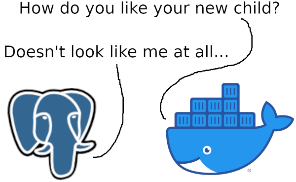
Laurenz Albe: Docker and sudden death for PostgreSQL
© Laurenz Albe 2023
This is a short war story from a customer problem. It serves as a warning that there are special considerations when running software in a Docker container.
The problem description
The customer is running PostgreSQL in Docker containers. They are not using the “official” image, but their own.
Sometimes, under conditions of high load, PostgreSQL crashes with
LOG:  server process (PID 84799) was terminated by signal 13: Broken pipe
LOG:  terminating any other active server processes
This causes PostgreSQL to undergo crash recovery, during which the service is not available.
Why crash recovery?
SIGPIPE (signal 13 on Linux) is a rather harmless signal: the kernel sends that signal to a process that tries to write to a pipe if the process at the other end of the pipe no longer exists. Crash recovery seems like a somewhat excessive reaction to that. If you look at the log entry, the message level is LOG and not PANIC (an error condition that PostgreSQL cannot recover from).
The reason for this excessive reaction is that PostgreSQL does not expect a child process to die from signal 13. A careful scrutiny of the PostgreSQL code shows that all PostgreSQL processes ignore SIGPIPE. So if one of these processes dies from that signal, something must be seriously out of order.
The role of the postmaster process
In PostgreSQL, the postmaster process (the parent of all server processes) listens for incoming connections and starts new server processes. It takes good care of its children: it respawns background processes that terminated in a controlled fashion, and it watches out for children that died from “unnatural causes”. Any such event is alarming, because all PostgreSQL processes use shared buffers, the shared memory segment that contains the authoritative copy of the table data. If a server process runs amok, it can scribble over these shared data and corrupt the database. Also, something could interrupt a server process in the middle of a “critical section” and leave the database in an inconsistent state. To prevent that from happening, the postmaster treats any irregular process termination as a sign of danger. Since shared buffers might be affected, the safe course is to interrupt processing and to restore consistency by performing crash recovery from the latest checkpoint.
(If this behavior strikes you as oversensitive, and you are less worried about data integrity, you might prefer more cavalier database systems like Oracle, where a server crash – euphemistically called ORA-00600 – does not trigger such a reaction.)
Hunting the rogue process in the Docker container
To understand and fix the problem, it was important to know which server process died from signal 13. All we knew is the process ID from the error message. We searched the log files for messages by this process, which is easy if you log the process ID with each entry. However, that process never left any trace in the log, even when we cranked up log_min_messages to debug3.
An added difficulty was that the error condition could not be reproduced on demand. All that we could do is to increase the load on the system by starting a backup, in the hope that the problem would manifest.
The next idea was to take regular “ps” snapshots in the hope to catch the offending process red-handed. The process remained elusive. Finally, the customer increased the frequency of those snapshots to one per second, and in the end we got a mug shot of our adversary.
The process turned out not to be a server process at all. Rather, it was a psql process that gets started inside the container to run a monitoring query on the database. Now psql is a client program that does not ignore SIGPIPE, so that mystery is solved. But how can psql be a PostgreSQL server process?
The ps snapshot that helped solve the Docker problem
The snapshot in question like this:
    PID STIME USER     COMMAND
      1 Mar13 postgres /usr/lib/postgresql/14/bin/postgres -D /postgresqldata/14
    332 Mar13 postgres postgres: logger
  84507 11:09 postgres postgres: checkpointer
  84508 11:09 postgres postgres: background writer
  84509 11:09 postgres postgres: walwriter
  84510 11:09 postgres postgres: autovacuum launcher
  84511 11:09 postgres postgres: archiver
  84512 11:09 postgres postgres: stats collector
  84513 11:09 postgres postgres: logical replication launcher
  84532 11:09 postgres postgres: logrep_user mydb 10.0.0.42(36270) idle
  84557 11:09 postgres postgres: postgres postgres 10.0.0.232(37434) idle
  84756 11:10 postgres postgres: appuser mydb 10.0.0.12(38600) idle
  84773 11:10 postgres postgres: appuser mydb 10.0.0.12(38610) idle
  84799 11:10 root     /usr/lib/postgresql/14/bin/psql -U postgres -t -c SELECT 1=1
The last line is the offending process, which is about to receive signal 13. This is very clearly not a server process; among other things, it is owned by the root user instead of postgres. Unfortunately, the snapshot does not include the parent process ID. However, since the postmaster (in the first line) recognized the rogue process as its child, it must be the parent.
Unplanned adoption in a Docker container
The key observation is that the process ID of the postmaster is 1. In Unix, process 1 is a special process: it is the first user land process that the kernel starts. This process then starts other processes to bring the system up. It is the ancestor of all other processes, and every other process has a parent process. There is another special property of process 1: if the parent process of a process dies, the kernel automatically assigns process 1 as parent to the orphaned process. Process 1 has to “adopt” all orphans.
Normally, process 1 is a special init executable specifically designed for this purpose. But in a Docker container, process 1 is the process that you executed to start the container. As you can see, that was the postmaster. The postmaster handles one of the tasks of the init process admirably: it waits for its children and collects the exit status when one of them dies. This keeps zombie processes from lingering for any length of time. However, the postmaster is less suited to handle another init task: remain stoic if one of its children dies horribly. That is what caused our problem.
How can we avoid this problem?
Once we understand the problem, the solution is simple: don’t start the container with PostgreSQL. Rather, start a different process, which in turn starts the postmaster. Either write your own or use an existing solution like dumb-init. The official PostgreSQL docker image does it right.
This problem also could not have occurred if the psql process hadn’t been started inside the container. It is good practice to consider a container running a service as a closed unit: you shouldn’t start jobs or interactive sessions inside the container. I can understand the appeal of using the container’s psql executable to avoid having to install the PostgreSQL client anywhere else, but it is a shortcut that you shouldn’t take.
Conclusion
It turned out that the cause of our problem was that the postmaster served as process 1 in the Docker container. The psql process that ran a monitoring query died from a SIGPIPE under high load. The postmaster, which had inadvertently inherited that process, noticed this unusual process termination and underwent crash recovery to stay on the safe side.
While running a program in a Docker container is not very different from running it outside in most respects, there are some differences that you have to be aware of if you want your systems to run stably.
You can read more about PostgreSQL and Docker in this article, “Running Postgres in Docker Why and How”.
The post Docker and sudden death for PostgreSQL appeared first on CYBERTEC.
Tesla Confirms Automated Driving Systems Were Engaged During Fatal Crash

Tesla has reportedly told U.S. regulators that a fatal crash involving a Model S earlier this year involved its automated driver-assist systems. According to Bloomberg, that’s the 17th fatal Tesla crash while the systems were engaged since June 2021. The number would likely be higher, save for the fact that the…
Philip Hurst: Introduction to Postgres Backups
Backups in the database world are essential. They are the safety net protecting you from even the smallest bit of data loss. There’s a variety of ways to back up your data and this post aims to explain the basic tools involved in backups and what options you have, from just getting started to more sophisticated production systems.
pg_dump/pg_restore
pg_dump and pg_dumpall are tools designed to generate a file and then allow
a database to be restored. These are classified as logical backups and they can
be much smaller in size than physical backups. This is due, in part, to the fact
that indexes are not stored in the SQL dump. Only the CREATE INDEX command is
stored and indexes must be rebuilt when restoring from a logical backup.
One advantage of the SQL dump approach is that the output can generally be reloaded into newer versions of Postgres so dump and restores are very popular for version upgrades and migrations. Another advantage is that these tools can be configured to back up specific database objects and ignore others. This is helpful, for example, if only a certain subset of tables need to be brought up in a test environment. Or you want to back up a single table as you do some risky work.
Postgres dumps are also internally consistent, which means the dump represents a snapshot of the database at the time the process started. Dumps will usually not block other operations, but they can be long-running (i.e. several hours or days, depending on hardware and database size). Because of the method Postgres uses to implement concurrency, known as Multiversion Concurrency Control, long running backups may cause Postgres to experience performance degradation until the dump completes.
To dump a single database table you can run something like:
pg_dump -t my_table > table.sql
To restore it, run something like:
psql -f table.sql
pg_dump as a corruption check
pg_dump sequentially scans through the entire data set as it creates the file.
Reading the entire database is a rudimentary corruption check for all the table
data, but not for indexes. If your data is corrupted, pg_dump will throw an
exception. Crunchy generally recommends using the
amcheck module to do a
corruption check, especially during some kind of upgrade or migration where
collations
might be involved.
Server & file system backups
If you’re coming from the Linux admin world, you’re used to backup options for
the entire machine your database runs on, using rsync or another tool.
Postgres cannot safely backup using file-oriented tools while it’s running, and
there’s not a simple way to quiesce writes either. To get the database into a
state where you can rsync the data, you either have to shut it down or go
through all the work of setting up change archiving. There are also some other
options for storage layers that support snapshots for the entire data
directory - but read the fine print on these.
Physical Backups & WAL archiving
Beyond basic dump files, the more sophisticated methods of Postgres backup all
depend on saving the database’s Write-Ahead-Log (WAL) files. WAL tracks changes
to all the database blocks, saving them into segments that default to 16MB in
size. The continuous set of a server’s WAL files are referred to as its WAL
stream. You have to start archiving the WAL stream’s files before you can safely
copy the database, followed by a procedure that produces a “Base Backup”, i.e.
pg_basebackup. The incremental aspect of WAL makes possible a series of other
restoration features lumped under the banner of
Point In Time Recovery
tools.
Create a basebackup with pg_basebackup:
You can use something like this:
$ sudo -u postgres pg_basebackup -h localhost -p 5432 -U postgres \
	-D /var/lib/pgsql/15/backups -Ft -z -Xs -P -c fast
A few comments on the command above.
- This command should be run as the
postgresuser. - The
-Dparameter specifies where to save the backup. - The
-Ftparameter indicates the tar format should be used. - The
-Xsparameter indicates that WAL files will stream to the backup. This is important because substantial WAL activity could occur while the backup is taken and you may not want to retain those files in the primary during this period. This is the default behavior, but worth pointing out. - The
-zparameter indicates that tar files will be compressed. - The
-Pparameter indicates that progress information is written to stdout during the process. - The
-cfast parameter indicates that a checkpoint is taken immediately. If this parameter is not specified, then the backup will not begin until Postgres issues a checkpoint on its own, and this could take a significant amount of time.
Once the command is entered, the backup should begin immediately. Depending upon the size of the cluster, it may take some time to finish. However, it will not interrupt any other connections to the database.
Steps to restore from a backup taken with pg_basebackup
They are simplified from the official documentation. If you are using some features like tablespaces you will need to modify these steps for your environment.
- Ensure the database is shutdown.
$ sudo systemctl stop postgresql-15.service
$ sudo systemctl status postgresql-15.service
- Remove the contents of the Postgres data directory to simulate the disaster.
$ sudo rm -rf /var/lib/pgsql/15/data/*
- Extract base.tar.gz into the data directory.
$ sudo -u postgres ls -l /var/lib/pgsql/15/backups
total 29016
-rw-------. 1 postgres postgres   182000 Nov 23 21:09 backup_manifest
-rw-------. 1 postgres postgres 29503703 Nov 23 21:09 base.tar.gz
-rw-------. 1 postgres postgres	17730 Nov 23 21:09 pg_wal.tar.gz


$ sudo -u postgres tar -xvf /var/lib/pgsql/15/backups/base.tar.gz \
     -C /var/lib/pgsql/15/data
- Extract pg_wal.tar.gz into a new directory outside the data directory. In our case, we create a directory called pg_wal inside our backups directory.
$ sudo -u postgres ls -l /var/lib/pgsql/15/backups
total 29016
-rw-------. 1 postgres postgres   182000 Nov 23 21:09 backup_manifest
-rw-------. 1 postgres postgres 29503703 Nov 23 21:09 base.tar.gz
-rw-------. 1 postgres postgres	17730 Nov 23 21:09 pg_wal.tar.gz

$ sudo -u postgres mkdir -p /var/lib/pgsql/15/backups/pg_wal

$ sudo -u postgres tar -xvf /var/lib/pgsql/15/backups/pg_wal.tar.gz \
      -C /var/lib/pgsql/15/backups/pg_wal/
- Create the recovery.signal file.
$ sudo -u postgres touch /var/lib/pgsql/15/data/recovery.signal
- Set the restore_command in postgresql.conf to copy the WAL files streamed during the backup.
$ echo "restore_command = 'cp /var/lib/pgsql/15/backups/pg_wal/%f %p'" | \
      sudo tee -a /var/lib/pgsql/15/data/postgresql.conf
- Start the database.
$ sudo systemctl start postgresql-15.service sudo systemctl status
postgresql-15.service
- Now your database is up and running based on the information contained in the previous basebackup.
Automating physical backups
Building upon the pg_basebackup, you could write a series of scripts to use
this backup, add WAL segments to it, and manage a complete physical backup
scenario. There are several tools out there including WAL-E, WAL-G, and
pgBackRest that will do all this for you. WAL-G is the next generation of WAL-E
and works for quite a few other databases including MySQL and Microsoft SQL
Server. WAL-G is also used extensively at the enterprise level with some large
Postgres environments, including Heroku. When we first built Crunchy Bridge, we
had a choice between WAL-G and pgBackRest since we employ the maintainers of
both and each has its perks. In the end, we selected pgBackRest.
pgBackRest
pgBackRest is the best in class backup tool out there. There are a number of very large Postgres environments relying on pgBackRest, including our own Crunchy Bridge, Crunchy for Kubernetes, and Crunchy Postgres as well as countless other projects in the Postgres ecosystem.
pgBackRest can perform three types of backups:
- Full backups - these copy the entire contents of the database cluster to the backup.
- Differential backups - this copies only the database cluster files that have changed since the last full backup
- Incremental backups - which copy only the database cluster files that have changed since the last full, differential, or incremental.
pgBackRest has some special features like:
- Allowing you to go back to a Point in Time - PITR (Point-in-Time Recovery)
- Creating a Delta Restore which will use database files already present and updated based on WAL segments. This makes potential restores much faster, especially if you have a large database and don’t want to restore the entire thing.
- Letting you have multiple backup repositories - say one local or one remote for redundancy.
Concerning archiving, users can set the archive_command parameter to use
pgBackRest to copy WAL files to an external archive. These files could be
retained indefinitely or expired in accordance with your organization's data
retention policies.
To start pgBackRest after installation, you’ll run something like this:
$ sudo -u postgres pgbackrest --stanza=demo --log-level-console=info stanza-create
To do a delta restore:
$ sudo systemctl stop postgresql-15.service
$ sudo -u postgres pgbackrest \
--stanza=db --delta \
--type=time "--target=2022-09-01 00:00:05.010329+00" \
--target-action=promote restore
When the restore completes, you restart the database and verify that the users table is back.
$ sudo systemctl start postgresql-15.service
$ sudo -u postgres psql -c "select * from users limit 1"
Backup timing
pgBackRest has pretty extensive settings and configurations to set up a strategy specific to your needs. Your backup strategy will depend on several factors, including the recovery point objective, available storage, and other factors. The right solution will vary based on these requirements. Finding the right strategy for your use case is a matter of striking a balance between the time to restore, the storage used, IO overhead on the source database, and other factors.
Our usual recommendation is to combine the backup and WAL archival capabilities of pgBackRest. We usually recommend customers take a weekly full base backup in addition to their continuous archiving of WAL files, and consider if other incremental backup forms--maybe even pg_dump--make sense for your requirements.
Conclusion
Choosing the backup tool for your use case will be a personal choice based on your needs, tolerance for recovery time, and available storage. In general, it is best to think of pg_dump is as a utility for doing specific database tasks. pg_basebackup can be an option if you’re ok with single physical backups on a specific time basis. If you have a production system of size and need to create a disaster recovery scenario, it's best to implement pgBackRest or a more sophisticated tool using WAL segments on top of a base backup. Of course, there’s fully managed options out there like Crunchy Bridge which will handle all this for you.
Co-authored with Elizabeth Christensen
An important next step on our AI journey
 Introducing Bard, Google's experimental conversational AI service powered by LaMDA — plus, new AI features in Search coming soon.
BYD Overcomes Tesla to Become World's Largest EV Maker

Chinese automaker BYD outsold Tesla by a wide margin last year with the help of its inexpensive electric cars. BYD has now become the biggest EV maker in the world, according to the South China Morning Post, but only when accounting for its sales of both fully-electric and plug-in hybrid models.
A simple stack for today's web hacks
Web development can be overwhelming, with frameworks and tools continually churning. Here's some advice that has worked well for me on my own projects which emphasizes simplicity, stability, and predictability. The recommendations I make here are only for tools that are high quality and which are unlikely to change significantly in the future.
Like most things I write on this blog, my intended audience is more or less "me if I didn't know this stuff already", so if you're say a C++ developer who isn't super familiar with nodejs etc and just wants to write a bit of TypeScript then this is the post for you. People have a lot of strong opinions about this stuff — to my mind, too strong, when a lot of the details really just don't matter that much, especially given how whimsical web fashion is — but if you are such a person then this post is certainly not for you!
To start with, we're not going to use any preconfigured template repository. Blog posts like this one seem to usually start with "copy my setup" but that feels like the opposite of what I want — I want the fewest moving parts possible and to be able understand what pieces I do use are for.
Instead we start from scratch:
$ mkdir myproject
$ cd myproject
Next, for frontend tooling, npm is inevitable. (Installing nodejs/npm is out of scope here since it's OS-dependent but it's trivial.) Make your project a root directory for npm dependencies, bypassing any questions:
$ npm init -y
This generates package.json. Most of its contents aren't necessary, feel free
to edit.
With npm in place we install TypeScript. I think of TypeScript as the bare minimum for keeping sane writing JS and it's a self-contained dependency. We install a copy of TypeScript per project because we want the TypeScript compiler version pinned to the project, which makes it resilient to bitrotting as new TypeScript versions come out.
$ npm install typescript
This downloads the compiler into the node_modules directory, updates
package.json, and adds package-lock.json, which records the pinned version
of the compiler.
Next we mark the repository as a TypeScript root.
$ npx tsc --init
Note the command there is npx, which means "run a binary found within the
local node_modules". tsc is the TypeScript compiler, and --init has it
generate a tsconfig.json, which configures the compiler. The bulk of this file
is commented out; the defaults are mostly fine. However, if you intend to use
any libraries from npm (see below) you will need to switch it from the default,
backward compatible module resolution to the more expected npm-compatible
behavior by uncommenting this line:
"moduleResolution": "node",
At this point if you create any .ts files, VSCode etc. will type-check them as
you edit. Running npx tsc will type-check and also convert .ts files to
.js.
Create some trivial inputs to try it out:
$ echo "document.write('hello, world');" > main.ts
$ echo "<script src='main.js'></script>" > index.html
Unfortunately, TypeScript is only responsible for single file translation, and by default generates imports in a format compatible with nodejs but not browsers. Any realistic web project will involve multiple source files or dependencies and will require one last tool, a "bundler".
Typically this is where tools like webpack get involved and your complexity budget is immediately blown. Instead, I recommend esbuild, which is (consistent with the spirit of this post) minimal, self-contained, and fast.
So add esbuild as a dependency, downloading a copy into node_modules:
$ npm install esbuild
We invoke esbuild in two ways: to generate an output bundle and while developing. (You really only need the former if you're just willing to run it after each edit, but it's pretty easy to do both and it saves needing some other tools.)
esbuild has no configuration file; it's managed solely through command-line flags. The command to generate a single-file bundle from an input file will look something like this:
$ npx esbuild --bundle --target=es2020 --sourcemap --outfile=main.js main.ts
This generates a file main.js by crawling imports found in the given input
file. The --sourcemap flag lets you debug .ts source in a browser. (You'll
want to add *.js and *.js.map to your .gitignore.)
You can just stick this command in a shell script or Makefile, or you can stick
it in your package.json in the scripts block:
"scripts": {
  "bundle": "esbuild --bundle --target=es2020 --sourcemap --outfile=main.js main.ts"
}
and invoke it via npm run bundle. (Note you don't need the npx prefix in the
package.json command, it knows to find the binary itself.)
Finally, the other way to use esbuild while developing is to have it run a web
server that automatically bundles when you reload the page. This means you can
save and hit reload to get updated output without needing to run any build
commands. It also means you will load the app via HTTP rather than the files
directly, which is necessary for some web APIs (like fetch) to work.
The esbuild command here is exactly like the above with the addition of one flag:
$ npx esbuild [above flags] --servedir=.
It will print a URL to load when you run it. This web server serves index.html
(and other files like *.css) verbatim, but specifically when the browser loads
main.js it will manage converting it from TypeScript.
Note that the esbuild command does not run any TypeScript checks. If your
editor isn't running TypeScript checking for you, you can still invoke npx tsc
yourself (and on CI). If you do so, I suggest twiddling tsconfig.json to
uncomment the
"noEmit": true,
line so that TypeScript doesn't emit any outputs — you want to use only one tool (esbuild) for this.
And with that, you're ready to go!
You might have some follow-up questions for recommendations which I will summarize in list form:
- Autoformatting. prettier is standard but clunky and is set up similarly to how other tools here have been set up. dprint is a newer replacement that I have liked more but it's newer and riskier.
- Linting. The current state of the ecosystem is a general mess, I suggest avoiding it.
- CSS languages. Too complex for my taste, possibly also because my projects tend to not be that visually complex.
- Web frameworks. This is a much more complex topic, worth an appendix!
Appendix: web frameworks.
The above is all you need to get started, but commonly the next thing you might want is to use some sort of web framework. There are a lot of these and depending on how fancy you get the framework itself will dictate its own versions of the above tools. A lot of the churn in web development is around frameworks, so if you're looking to stay simple and predictable adopting any of them is probably not the path you want.
But if you're again looking to stay simple and predictable, I have been happy with Preact, which is an API-compatible implementation of the industry-dominant React framework that is only 3kb. Unlike the above recommendations, I would note there's more potential for churn if you depend on Preact. But one nice property of Preact in particular is that it's intended to be a simpler React so it has a combination of limited API (due to small size) and well-understood standard API.
To modify the above project to use Preact, you need to install it:
$ npm install preact
Rename main.ts into main.tsx and update the build commands to refer to the
new path.
Tell TypeScript/esbuild to interpret the .tsx file as preact by changing two
settings within tsconfig.json:
"jsx": "react-jsx",
"jsxImportSource": "preact",
For completeness, I'll change the source files to a preact hello-world. Add a
body tag to index.html:
<body></body>
<script src='main.js'></script>
And call into preact from main.tsx:
import * as preact from 'preact';

preact.render(<h1>hello, world</h1>, document.body);
That ends up enough for most things I do, hope it works for you!
Monsters Are Everywhere in the Bible—And Some Are Even Human
This story was originally published on The Conversation and appears here under a Creative Commons license.
What is a “monster”? For most Americans, this word sparks images of haunted houses and horror movies: scary creations, neither human nor animal, and usually evil. But it can be helpful to think about “monsters” beyond these knee-jerk images. Ever since the 1990s, humanities scholars have been paying close attention to “monstrous” bodies in literature: characters whose appearance challenges common ideas about what’s normal.
Biblical scholars like me have followed in their footsteps. The Bible is full of monsters, even if they’re not Frankenstein or Bigfoot, and these characters can teach important lessons about ancient authors, texts and cultures. Monsterlike characters—even human ones—can convey ideas about what’s considered normal and good or “deviant,” disturbing, and evil.
Sometimes, monsters’ bodies are depicted in ways that reflect racist or sexist stereotypes about “us” versus “them.” Literary theorist Jack Halberstam, for example, has written about how Dracula and other vampires reveal antisemitic symbolism—even on Count Chocula cereal boxes. Such images often draw on antisemitic tropes that have been around for centuries, portraying Jewish people as shadowy, bloodsucking parasites.
Biblical monsters are no less revealing. In the Book of Judges, for example, the judge Ehud confronts the grotesque Moabite king Eglon, who is fatally fat and dies in an explosion of his own feces when a sword gets stuck in his stomach–though most modern translations render this a bit more chastely: “[Eglon’s] fat closed over [Ehud’s] blade, and the hilt went in after the blade—for he did not pull the dagger out of his belly—and the filth came out.”
In describing Eglon, the text also teaches Israelites how to think about their Moabite neighbors across the Jordan River. Like their emblematic king, Moabites are portrayed as excessive and disgusting—but ridiculous enough that Israelite heroes can defeat them with a few tricks.
Figures like Eglon and the famous Philistine giant Goliath, who battles the future King David, offer opportunities for biblical authors to subtly instruct readers about other groups of people that the authors consider threatening or inferior. But the Bible sometimes draws a relatable human character and then inserts twists, playing with the audience’s expectations.

In my own recent work, I have suggested that this is exactly what’s going on with the Book of Job. In this mostly poetic book of the Bible, “The Satan” claims that Job acts righteously only because he is prosperous and healthy. God grants permission for the fiend to test Job by causing his children to be killed, his livestock to be stolen and his body to break out in painful boils.
Job is then approached by three friends, who insist that he must have done something to prompt this apparent punishment. He spends the rest of the book debating with them about the cause of his torment.
The book is full of monsters and already a familiar topic in monster studies. In chapters 40-41, God boasts about two superanimals that he has created, called Leviathan and Behemoth. A mysterious, possibly maritime monster called Rahab appears twice. Both Job and his friends refer to vague nighttime visions that terrify them.
And of course there’s another “monster,” too: Job’s test is instigated by “the Satan.” Later in history, this figure became the archfiend of Jewish and Christian theology. In the Book of Job, though, he’s simply portrayed as a crooked minion, a shifty member of God’s heavenly court.
But I’d argue there’s another “monster” hiding in plain sight: the man at the center of it all. As biblical scholars like Rebecca Raphael and Katherine Southwood have pointed out, Job’s body is central to the book’s plot.
Job stoically tolerates Satan’s attacks on his livestock and even his children. It is only after the second attack, which produces “a severe inflammation on Job from the sole of his foot to the crown of his head,” that he lets out a deluge of complaints.
Job’s body is so transformed that he, too, can be seen as a “monster.”
To illustrate his suffering, Job repeatedly describes his bodily decay with macabre, gruesome images: “My skin, blackened, is peeling off me. My bones are charred by the heat.” And, “My flesh is covered with maggots and clods of earth; My skin is broken and festering.” Job’s body is so transformed that he, too, can be seen as a “monster.” But while Job might think that the deity prefers ideal human bodies, this is not necessarily the case.
In the book’s telling, God sustains unique, extraordinary monsters who would seem, at first glance, to be evil or repellent—but actually serve as prime examples of creation’s wonder and diversity. And it is Satan, not God, who decides to test Job by afflicting him physically.
Some books in the Bible indeed view monsters as simplistic, inherently evil “others.” The prophet Daniel, for example, has visions of four hybrid beasts, including a winged lion and a multiheaded leopard. These were meant to symbolize threatening ancient empires that the chapter’s author despised.
The Book of Job does something radical by pushing against this limited view. Its inclusive viewpoint portrays the “monstrous” human as a sympathetic character who has his place in a diverse, chaotic world—challenging readers’ preconceptions today, just as it might have thousands of years ago.
Madadh Richey is an assistant professor of Hebrew Bible at Brandeis University.
Ryan Booz: How We Made Data Aggregation Better and Faster on PostgreSQL With TimescaleDB 2.7
It’s time for another #AlwaysBeLaunching week! 🥳🚀✨ In our #AlwaysBeLaunching initiatives, we challenge ourselves to bring you an array of new features and content. Today, we are introducing TimescaleDB 2.7 and the performance boost it brings for aggregate queries. 🔥 Expect more news this week about further performance improvements, developer productivity, SQL, and more. Make sure you follow us on Twitter (@TimescaleDB), so you don’t miss any of it!
Time-series data is the lifeblood of the analytics revolution in nearly every industry today. One of the most difficult challenges for application developers and data scientists is aggregating data efficiently without always having to query billions (or trillions) of raw data rows. Over the years, developers and databases have created numerous ways to solve this problem, usually similar to one of the following options:
- DIY processes to pre-aggregate data and store it in regular tables. Although this provides a lot of flexibility, particularly with indexing and data retention, it's cumbersome to develop and maintain, particularly deciding how to track and update aggregates with data that arrives late or has been updated in the past.
- Extract Transform and Load (ETL) process for longer-term analytics. Even today, development teams employ entire groups that specifically manage ETL processes for databases and applications because of the constant overhead of creating and maintaining the perfect process.
- MATERIALIZED VIEWS. While these VIEWS are flexible and easy to create, they are static snapshots of the aggregated data. Unfortunately, developers need to manage updates using TRIGGERs or CRON-like applications in all current implementations. And in all but a very few databases, all historical data is replaced each time, preventing developers from dropping older raw data to save space and computation resources every time the data is refreshed.
Most developers head down one of these paths because we learn, often the hard way, that running reports and analytic queries over the same raw data, request after request, doesn't perform well under heavy load. In truth, most raw time-series data doesn't change after it's been saved, so these complex aggregate calculations return the same results each time.
In fact, as a long-term time-series database developer, I've used all of these methods too, so that I could manage historical aggregate data to make reporting, dashboards, and analytics faster and more valuable, even under heavy usage.
I loved when customers were happy, even if it meant a significant amount of work behind the scenes maintaining that data.
But, I always wished for a more straightforward solution.
How TimescaleDB Improves Queries on Aggregated Data in PostgreSQL
In 2019, TimescaleDB introduced continuous aggregates to solve this very problem, making the ongoing aggregation of massive time-series data easy and flexible. This is the feature that first caught my attention as a PostgreSQL developer looking to build more scalable time-series applications—precisely because I had been doing it the hard way for so long.
Continuous aggregates look and act like materialized views in PostgreSQL, but with many of the additional features I was looking for. These are just some of the things they do:
- Automatically track changes and additions to the underlying raw data.
- Provide configurable, user-defined policies to keep the materialized data up-to-date automatically.
- Automatically append new data (as real-time aggregates by default) before the scheduled process has materialized to disk. This setting is configurable.
- Retain historical aggregated data even if the underlying raw data is dropped.
- Can be compressed to reduce storage needs and further improve the performance of analytic queries.
- Keep dashboards and reports running smoothly.

Once I tried continuous aggregates, I realized that TimescaleDB provided the solution that I (and many other PostgreSQL users) were looking for. With this feature, managing and analyzing massive volumes of time-series data in PostgreSQL finally felt fast and easy.
What About Other Databases?
By now, some readers might be thinking something along these lines:
“Continuous aggregates may help with the management and analytics of time-series data in PostgreSQL, but that’s what NoSQL databases are for—they already provide the features you needed from the get-go. Why didn’t you try a NoSQL database?”
Well, I did.
There are numerous time-series and NoSQL databases on the market that attempt to solve this specific problem. I looked at (and used) many of them. But from my experience, nothing can quite match the advantages of a relational database with a feature like continuous aggregates for time-series data. These other options provide a lot of features for a myriad of use cases, but they weren't the right solution for this particular problem, among other things.
What about MongoDB?
MongoDB has been the go-to for many data-intensive applications. Included since version 4.2 is a feature called On-Demand Materialized Views. On the surface, it works similar to a materialized view by combining the Aggregation Pipeline feature with a $merge operation to mimic ongoing updates to an aggregate data collection. However, there is no built-in automation for this process, and MongoDB doesn't keep track of any modifications to underlying data. The developer is still required to keep track of which time frames to materialize and how far back to look.
What about InfluxDB?
For many years InfluxDB has been the destination for time-series applications. Although we've discussed in other articles how InfluxDB doesn't scale effectively, particularly with high cardinality datasets, it does provide a feature called Continuous Queries. This feature is also similar to a materialized view and goes one step further than MongoDB by automatically keeping the dataset updated. Unfortunately, it suffers from the same lack of raw data monitoring and doesn't provide nearly as much flexibility as SQL in how the datasets are created and stored.
What about Clickhouse?
Clickhouse, and several recent forks like Firebolt, have redefined the way some analytic workloads perform. Even with some of the impressive query performance, it provides a mechanism similar to a materialized view as well, backed by an AggregationMergeTree engine. In a sense, this provides almost real-time aggregated data because all inserts are saved to both the regular table and the materialized view. The biggest downside of this approach is dealing with updates or modifying the timing of the process.
Recent Improvements in Continuous Aggregates: Meet TimescaleDB 2.7
Continuous aggregates were first introduced in TimescaleDB 1.3 solving the problems that many PostgreSQL users, including me, faced with time-series data and materialized views: automatic updates, real-time results, easy data management, and the option of using the view for downsampling.
But continuous aggregates have come a long way. One of the previous improvements was the introduction of compression for continuous aggregates in TimescaleDB 2.6. Now, we took it a step further with the arrival of TimescaleDB 2.7, which introduces dramatic performance improvements in continuous aggregates. They are now blazing fast—up to 44,000x faster in some queries than in previous versions.
Let me give you one concrete example: in initial testing using live, real-time stock trade transaction data, typical candlestick aggregates were nearly 2,800x faster to query than in previous versions of continuous aggregates (which were already fast!)

Later in this post, we will dig into the performance and storage improvements introduced by TimescaleDB 2.7 by presenting a complete benchmark of continuous aggregates using multiple datasets and queries. 🔥
But the improvements don’t end here.
First, the new continuous aggregates also require 60 % less storage (on average) than before for many common aggregates, which directly translates into storage savings.
Second, in previous versions of TimescaleDB, continuous aggregates came with certain limitations: users, for example, could not use certain functions like DISTINCT, FILTER, or ORDER BY. These limitations are now gone. TimescaleDB 2.7 ships with a completely redesigned materialization process that solves many of the previous usability issues, so you can use any aggregate function to define your continuous aggregate. Check out our release notes for all the details on what's new.
And now, the fun part.
Show Me the Numbers: Benchmarking Aggregate Queries
To test the new version of continuous aggregates, we chose two datasets that represent common time-series datasets: IoT and financial analysis.
- IoT dataset (~1.7 billion rows): The IoT data we leveraged is the New York City Taxicab dataset that's been maintained by Todd Schneider for a number of years, and scripts are available in his GitHub repository to load data into PostgreSQL. Unfortunately, a week after his latest update, the transit authority that maintains the actual datasets changed their long-standing export data format from CSV to Parquet—which means the current scripts will not work. Therefore, the dataset we tested with is from data prior to that change and covers ride information from 2014 to 2021.
- Stock transactions dataset (~23.7 million rows): The financial dataset we used is a real-time stock trade dataset provided by Twelve Data and ingests ongoing transactions for the top 100 stocks by volume from February 2022 until now. Real-time transaction data is typically the source of many stock trading analysis applications requiring aggregate rollups over intervals for visualizations like candlestick charts and machine learning analysis. While our example dataset is smaller than a full-fledged financial application would maintain, it provides a working example of ongoing data ingestion using continuous aggregates, TimescaleDB native compression, and automated raw data retention (while keeping aggregate data for long-term analysis).
You can use a sample of this data, generously provided by Twelve Data, to try all of the improvements in TimescaleDB 2.7 by following this tutorial, which provides stock trade data for the last 30 days. Once you have the database setup, you can take it a step further by registering for an API key and following our tutorial to ingest ongoing transactions from the Twelve Data API.
Creating Continuous Aggregates Using Standard PostgreSQL Aggregate Functions
The first thing we benchmarked was to create an aggregate query that used standard PostgreSQL aggregate functions like MIN(), MAX(), and AVG(). In each dataset we tested, we created the same continuous aggregate in TimescaleDB 2.6.1 and 2.7, ensuring that both aggregates had computed and stored the same number of rows.
IoT dataset
This continuous aggregate resulted in 1,760,000 rows of aggregated data spanning seven years of data.
CREATE MATERIALIZED VIEW hourly_trip_stats
WITH (timescaledb.continuous, timescaledb.finalized=false)
AS
SELECT
	time_bucket('1 hour',pickup_datetime) bucket,
	avg(fare_amount) avg_fare,
	min(fare_amount) min_fare,
	max(fare_amount) max_fare,
	avg(trip_distance) avg_distance,
	min(trip_distance) min_distance,
	max(trip_distance) max_distance,
	avg(congestion_surcharge) avg_surcharge,
	min(congestion_surcharge) min_surcharge,
	max(congestion_surcharge) max_surcharge,
	cab_type_id,
	passenger_count
FROM
	trips
GROUP BY
	bucket, cab_type_id, passenger_count
Stock transactions dataset
This continuous aggregate resulted in 950,000 rows of data at the time of testing, although these are updated as new data comes in.
CREATE MATERIALIZED VIEW five_minute_candle_delta
WITH (timescaledb.continuous) AS
    SELECT
        time_bucket('5 minute', time) AS bucket,
        symbol,
        FIRST(price, time) AS "open",
        MAX(price) AS high,
        MIN(price) AS low,
        LAST(price, time) AS "close",
        MAX(day_volume) AS day_volume,
        (LAST(price, time)-FIRST(price, time))/FIRST(price, time) AS change_pct
    FROM stocks_real_time srt
    GROUP BY bucket, symbol;
To test the performance of these two continuous aggregates, we selected the following queries, all common queries among our users for both the IoT and financial use cases:
- SELECT COUNT (*)
- SELECT COUNT (*) with WHERE
- ORDER BY
- time_bucket reaggregation
- FILTER
- HAVING
Let’s take a look at the results.
Query #1: `SELECT COUNT(*) FROM…`
Doing a COUNT(*) from PostgreSQL is a known performance bottleneck. It's one of the reasons we created the approximate_row_count() function in TimescaleDB which uses table statistics to provide a close approximation of the overall row count. However, it's instinctual for most users (and ourselves, if we're honest) to try and get a quick row count by doing a COUNT(*) query:
-- IoT dataset
SELECT count(*) FROM hourly_trip_stats;

-- Stock transactions dataset
SELECT count(*) FROM five_min_candle_delta;
And most users recognized that in previous versions of TimescaleDB, the materialized data seemed slower than normal to do a COUNT over.
Thinking about our two example datasets, both continuous aggregates reduce the overall row count from raw data by 20x or more. So, while counting rows in PostgreSQL is slow, it always felt a little slower than it had to be. The reason was that not only did PostgreSQL have to scan and count all of the rows of data, it had to group the data a second time because of some additional data that TimescaleDB stored as part of the original design of continuous aggregates. With the new design of continuous aggregates in TimescaleDB 2.7, that second grouping is no longer required, and PostgreSQL can just query the data normally, translating into faster queries.

Query #2: SELECT COUNT(*) Based on The Value of a Column
Another common query that many analytic applications perform is to count the number of records where the aggregate value is within a certain range:
-- IoT  dataset
SELECT count(*) FROM hourly_trip_stats
WHERE avg_fare > 13.1
AND bucket > '2018-01-01' AND bucket < '2019-01-01';

-- Stock transactions dataset
SELECT count(*) FROM five_min_candle_delta
WHERE change_pct > 0.02;
In previous versions of continuous aggregates, TimescaleDB had to finalize the value before it could be filtered against the predicate value, which caused queries to perform more slowly. With the new version of continuous aggregates, PostgreSQL can now search for the value directly, and we can add an index to meaningful columns to speed up the query even more!
In the case of the financial dataset, we see a very significant improvement: 1,336x faster. The large change in performance can be attributed to the formula query that has to be calculated over all of the rows of data in the continuous aggregate. With the IoT dataset, we're comparing against a simple average function, but for the stock data, multiple values have to be finalized (FIRST/LAST) before the formula can be calculated and used for the filter.

Query #3: Select Top 10 Rows by Value
Taking the first example a step further, it's very common to query data within a range of time and get the top rows:
-- IoT dataset
SELECT * FROM hourly_trip_stats
ORDER BY avg_fare desc
LIMIT 10;

-- Stock transactions dataset
SELECT * FROM five_min_candle_delta
ORDER BY change_pct DESC
LIMIT 10;
In this case, we tested queries with the continuous aggregate set to provide real-time results (the default for continuous aggregates) and materialized-only results. When set to real-time, TimescaleDB always queries data that's been materialized first and then appends (with a UNION) any newer data that exists in the raw data but that has not yet been materialized by the ongoing refresh policy. And, because it's now possible to index columns within the continuous aggregate, we added an index on the ORDER BY column.

Yes, you read that correctly. Nearly 45,000x better performance on ORDER BY when the query only searches through materialized data.
The dramatic difference between real-time and materialized-only queries is because of the UNION of both materialized and raw aggregate data. The PostgreSQL planner needs to union the total result before it can limit the query to 10 rows (in our example), and so all of the data from both tables need to be read and ordered first. When you only query materialized data, PostgreSQL and TimescaleDB knows that it can query just the index of the materialized data.
Again, storing the finalized form of your data and indexing column values dramatically impacts the querying performance of historical aggregate data! And all of this is updated continuously over time in a non-destructive way—something that's impossible to do with any other relational database, including vanilla PostgreSQL.
Query #4: Timescale Hyperfunctions to Re-aggregate Into Higher Time Buckets
Another example we wanted to test was the impact finalizing data values has on our suite of analytical hyperfunctions. Many of the hyperfunctions we provide as part of the TimescaleDB Toolkit utilize custom aggregate values that allow many different values to be accessed later depending on the needs of an application or report. Furthermore, these aggregate values can be re-aggregated into different size time buckets. This means that if the aggregate functions fit your use case, one continuous aggregate can produce results for many different time_bucket sizes! This is a feature many users have asked for over time, and hyperfunctions make this possible.
For this example, we only examined the New York City Taxicab dataset to benchmark the impact of finalized CAGGs. Currently, there is not an aggregate hyperfunction that aligns with the OHLC values needed for the stock data set, however, there is a feature request for it! (😉)
Although there are not currently any one-to-one hyperfunctions that provide exact replacements for our min/max/avg example, we can still observe the query improvement using a tdigest value for each of the columns in our original query.
Original min/max/avg continuous aggregate for multiple columns:
CREATE MATERIALIZED VIEW hourly_trip_stats
WITH (timescaledb.continuous, timescaledb.finalized=false)
AS
SELECT
	time_bucket('1 hour',pickup_datetime) bucket,
	avg(fare_amount) avg_fare,
	min(fare_amount) min_fare,
	max(fare_amount) max_fare,
	avg(trip_distance) avg_distance,
	min(trip_distance) min_distance,
	max(trip_distance) max_distance,
	avg(congestion_surcharge) avg_surcharge,
	min(congestion_surcharge) min_surcharge,
	max(congestion_surcharge) max_surcharge,
	cab_type_id,
	passenger_count
FROM
	trips
GROUP BY
	bucket, cab_type_id, passenger_count
Hyperfunction-based continuous aggregate for multiple columns:
CREATE MATERIALIZED VIEW hourly_trip_stats_toolkit
WITH (timescaledb.continuous, timescaledb.finalized=false)
AS
SELECT
	time_bucket('1 hour',pickup_datetime) bucket,
	tdigest(1,fare_amount) fare_digest,
	tdigest(1,trip_distance) distance_digest,
	tdigest(1,congestion_surcharge) surcharge_digest,
	cab_type_id,
	passenger_count
FROM
	trips
GROUP BY
	bucket, cab_type_id, passenger_count
With the continuous aggregate created, we then queried this data in two different ways:
1. Using the same `time_bucket()` size defined in the continuous aggregate, which in this example was one-hour data.
SELECT
	bucket AS b,
	cab_type_id,
	passenger_count,
	min_val(ROLLUP(fare_digest)),
	max_val(ROLLUP(fare_digest)),
	mean(ROLLUP(fare_digest))
FROM hourly_trip_stats_toolkit
WHERE bucket > '2021-05-01' AND bucket < '2021-06-01'
GROUP BY b, cab_type_id, passenger_count
ORDER BY b DESC, cab_type_id, passenger_count;
2. We re-aggregated the data from one-hour buckets into one-day buckets. This allows us to efficiently query different bucket lengths based on the original bucket size of the continuous aggregate.
SELECT
	time_bucket('1 day', bucket) AS b,
	cab_type_id,
	passenger_count,
	min_val(ROLLUP(fare_digest)),
	max_val(ROLLUP(fare_digest)),
	mean(ROLLUP(fare_digest))
FROM hourly_trip_stats_toolkit
WHERE bucket > '2021-05-01' AND bucket < '2021-06-01'
GROUP BY b, cab_type_id, passenger_count
ORDER BY b DESC, cab_type_id, passenger_count;
In this case, the speed is almost identical because the same amount of data has to be queried. But if these aggregates satisfy your data requirements, only one continuous aggregate would be necessary in many cases, rather than a different continuous aggregate for each bucket size (one minute, five minutes, one hour, etc.)
Query #5: Pivot Queries With FILTER
In previous versions of continuous aggregates, many common SQL features were not permitted because of how the partial data was stored and finalized later. Using a PostgreSQL FILTER clause was one such restriction.
For example, we took the IoT dataset and created a simple COUNT(*) to calculate each company's number of taxi rides ( cab_type_id) for each hour. Before TimescaleDB 2.7, you would have to store this data in a narrow column format, storing a row in the continuous aggregate for each cab type.
CREATE MATERIALIZED VIEW hourly_ride_counts_by_type
WITH (timescaledb.continuous, timescaledb.finalized=false)
AS
SELECT
	time_bucket('1 hour',pickup_datetime) bucket,
	cab_type_id,
  	COUNT(*)
FROM trips
  	WHERE cab_type_id IN (1,2)
GROUP BY
	bucket, cab_type_id;
To then query this data in a pivoted fashion, we could FILTER the continuous aggregate data after the fact.
SELECT bucket,
	sum(count) FILTER (WHERE cab_type_id IN (1)) yellow_cab_count,
  	sum(count) FILTER (WHERE cab_type_id IN (2)) green_cab_count
FROM hourly_ride_counts_by_type
WHERE bucket > '2021-05-01' AND bucket < '2021-06-01'
GROUP BY bucket
ORDER BY bucket;
In TimescaleDB 2.7, you can now store the aggregated data using a FILTER clause to achieve the same result in one step!
CREATE MATERIALIZED VIEW hourly_ride_counts_by_type_new
WITH (timescaledb.continuous)
AS
SELECT
	time_bucket('1 hour',pickup_datetime) bucket,
  	COUNT(*) FILTER (WHERE cab_type_id IN (1)) yellow_cab_count,
  	COUNT(*) FILTER (WHERE cab_type_id IN (2)) green_cab_count
FROM trips
GROUP BY
	bucket;
Querying this data is much simpler, too, because the data is already pivoted and finalized.
SELECT * FROM hourly_ride_counts_by_type_new
WHERE bucket > '2021-05-01' AND bucket < '2021-06-01'
ORDER BY bucket;
This saves storage (50 % fewer rows in this case) and CPU to finalize the COUNT(*) and then filter the results each time based on cab_type_id. We can see this in the query performance numbers.

Being able to use FILTER and other SQL features improve both developer experience and flexibility long term!
Query #6: HAVING Stores Significantly Less Materialized Data
As a final example of how the improvements to continuous aggregates will impact your day-to-day development and analytics processes, let's look at a simple query that uses a HAVING clause to reduce the number of rows that the aggregate stores.
In previous versions of TimescaleDB, the having clause couldn't be applied at materialization time. Instead, the HAVING clause was applied after the fact to all of the aggregated data as it was finalized. In many cases, this dramatically affected both the speed of queries to the continuous aggregate and the amount of data stored overall.
Using our stock data as an example, let's create a continuous aggregate that only stores a row of data if the change_pct value is greater than 20 %. This would indicate that a stock price changed dramatically over one hour, something we don't expect to see in most hourly stock trades.
CREATE MATERIALIZED VIEW one_hour_outliers
WITH (timescaledb.continuous) AS
    SELECT
        time_bucket('1 hour', time) AS bucket,
        symbol,
        FIRST(price, time) AS "open",
        MAX(price) AS high,
        MIN(price) AS low,
        LAST(price, time) AS "close",
        MAX(day_volume) AS day_volume,
        (LAST(price, time)-FIRST(price, time))/LAST(price, time) AS change_pct
    FROM stocks_real_time srt
    GROUP BY bucket, symbol
   HAVING (LAST(price, time)-FIRST(price, time))/LAST(price, time) > .02;
Once the dataset is created, we can query each aggregate to see how many rows matched our criteria.
SELECT count(*) FROM one_hour_outliers;
The biggest difference here (and the one that will more negatively impact the performance of your application over time) is the storage size of this aggregated data. Because TimescaleDB 2.7 only stores rows that meet the criteria, the data footprint is significantly smaller!

Storage Savings in TimescaleDB 2.7
One of the final pieces of this update that excites us is how much storage will be saved over time. On many occasions, users with large datasets that contained complex equations in their continuous aggregates would join our Slack community to ask why more storage is required for the rolled-up aggregate than the raw data.
In every case we've tested, the new, finalized form of continuous aggregates is smaller than the same example in previous versions of TimescaleDB, with or without a HAVING clause that might filter additional data out.

The New Continuous Aggregates Are a Game-Changer
For those dealing with massive amounts of time-series data, continuous aggregates are the best way to solve a problem that has long haunted PostgreSQL users. The following list details how continuous aggregates expand materialized views:
- They always stay up-to-date, automatically tracking changes in the source table for targeted, efficient updates of materialized data.
- You can use configurable policies to conveniently manage refresh/update interval.
- You can keep your materialized data even after the raw data is dropped, allowing you to downsample your large datasets.
- And you can compress older data to save space and improve analytic queries.
And in TimescaleDB 2.7, continuous aggregates got much better. First, they are blazing fast: as we demonstrated with our benchmark, the performance of continuous aggregates got consistently better across queries and datasets, up to thousands of times better for common queries. They also got lighter, requiring an average of 60 % less storage.
But besides the performance improvements and storage savings, there are significantly fewer limitations on the types of aggregate queries you can use with continuous aggregates, such as:
- Aggregates with DISTINCT
- Aggregates with FILTER
- Aggregates with FILTER in HAVING clause
- Aggregates without combine function
- Ordered-set aggregates
- Hypothetical-set aggregates
This new version of continuous aggregates is available by default in TimescaleDB 2.7: now, when you create a new continuous aggregate, you will automatically benefit from all the latest changes. For your existing continuous aggregates, we recommend that you recreate them in the latest version to take advantage of all these improvements. Read our release notes for more information on TimescaleDB 2.7, and for instructions on how to upgrade, check out our docs.
☁️🐯 Timescale Cloud avoids the manual work involved in updating your TimescaleDB version. Updates take place automatically during a maintenance window picked by you. Learn more about automatic version updates in Timescale Cloud and start a free trial to test it yourself.