Shared posts

05 Feb 07:07

Scary Compiler Code Motion

by regehr

I ran across this blog post about reader-writer locks and thought it would be fun to present them to the Advanced Operating Systems class that I’m running this spring. Here’s my version of the code, which needed to be adapted a bit to work with GCC:

struct RWSpinLock
{
  volatile uint32_t lock;
};

void LockReader(struct RWSpinLock *l)
{
  while (1) {
    uint32_t OldLock = l->lock & 0x7fffffff;
    uint32_t NewLock = OldLock + 1;   
    if (__sync_val_compare_and_swap(&l->lock, OldLock, NewLock) == OldLock) 
      return;
  }
}
  
void UnlockReader(struct RWSpinLock *l)
{
  __sync_sub_and_fetch(&l->lock, 1);
}

void LockWriter(struct RWSpinLock *l)
{
 again:
  {
    uint32_t OldLock = l->lock & 0x7fffffff;
    uint32_t NewLock = OldLock | 0x80000000;    
    if (!(__sync_val_compare_and_swap(&l->lock, OldLock, NewLock) == OldLock)) 
      goto again;
    while (l->lock & 0x7fffffff) { }
  }
}

void UnlockWriter(struct RWSpinLock *l)
{
  l->lock = 0;
}

At first I was suspicious that some sort of fence is required in the UnlockWriter() function. However, I believe that that is not the case: TSO will naturally make sure that all cores see operations inside the locked region prior to seeing the lock release. On some non-TSO platforms this unlock function would be too weak.

But the hardware is only one source of reordering that can mess up locks — the compiler is another. The store to the volatile lock field in UnlockWriter() cannot be moved around another access to a volatile-qualified object, but (in my reading of the standard) stores to non-volatile objects can be moved around stores to volatiles.

Can we get a compiler to translate the (in principle) broken code into assembly that actually doesn’t work? Turns out this is easy:

int important_data;
struct RWSpinLock l;

void update (void)
{
  LockWriter (&l);
  important_data /= 20;
  UnlockWriter (&l);
}

Using the default compiler on an x86-64 Ubuntu 12.04 machine (GCC 4.6.3) at -O2, the resulting assembly is:

update:
	movl	$l, %edi
	call	LockWriter
	movl	important_data(%rip), %ecx
	movl	$1717986919, %edx
	movl	$0, l(%rip)
	movl	%ecx, %eax
	sarl	$31, %ecx
	imull	%edx
	sarl	$3, %edx
	subl	%ecx, %edx
	movl	%edx, important_data(%rip)
	ret

Notice that important_data is read inside the lock and written well outside of it. Yikes! Here’s how to stop the compiler from doing that:

void UnlockWriter(struct RWSpinLock *l)
{
  // this is necessary or else GCC will move operations out of the locked region
  asm volatile("" ::: "memory");
  l->lock = 0;
}

Versions of Clang that I tried (3.3 and 3.4 for x86-64) didn’t want to move the store to important_data outside of the lock, but it’s possible that I just wasn’t asking the right way.

05 Feb 07:06

PRESENTING LEVEL UP! SECOND EDITION!

by Scott Rogers


Wiley & Sons is publishing a SECOND EDITION of Level Up!

Since Level Up!'s release in 2010, the game industry has evolved with the rise of mobile gaming, social gaming, monetization and touch controls. (to name a few) Level Up! 2nd edition has been completely revised to address these topics and more - expanding on everything in the first edition. There's even a new introduction by God of War's David Jaffe, new artwork and a delicious new chili recipe! I hope you'll find Level Up! 2nd edition a home on your game design bookshelf.

Level Up! Second Edition will be released this summer everywhere books and e-books are sold.


05 Feb 07:01

Process Tree from an Xperf Trace

by brucedawson

I was looking at an xperf (ETW) trace recently and needed to know who had started a particular process. The parent process ID was stored in the trace so I could find its parent, and its parent’s parent, and so on, but doing this for many generations in WPA is tedious.

Luckily the 8.1 version of the Windows Performance Toolkit has a tool for exporting arbitrary data, so I used that and a bit of Python to write a tool that would create a process tree for an ETW trace.


The process export process

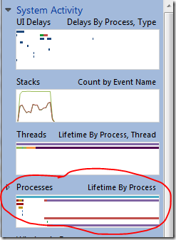
imageThe process of exporting process data starts with configuring WPA so that it displays the process data that I want to export. To do this I closed all of the open WPA graphs and tables and opened the Processes graph, found under System Activity in the graph explorer – see the screenshot at the right. I put the Processes graph into Table Only mode (Ctrl+Shift+T) because the graph isn’t relevant for exporting.

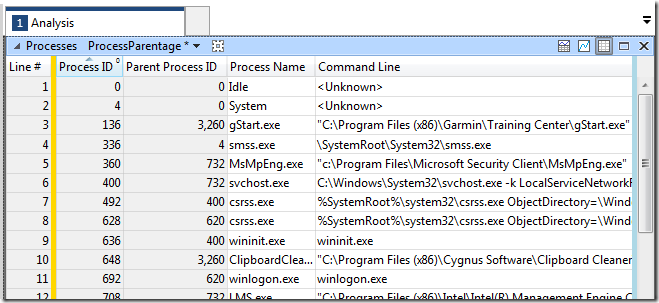
Then it was just a matter of selecting and rearranging the columns that I wanted into the order that I wanted them. It made sense to have Process ID and Parent Process ID first, so that my script could easily find them. The remaining columns I treat as data payload and they can be rearranged any way you want. I ended up with something like this:

image

You can export this profile from WPA using the Export command in the Profile menu. It’s kind of obvious when you say it like that. You can then apply the profile to a loaded trace using the Apply command in the Profile menu, but we’re going to use the profile for exporting data.

I saved my profile as XperfProcessPercentage.wpaProfile.

Export made easy

Exporting the data is as simple as running this command:

wpaexporter  mytrace.etl  XperfProcessParentage.wpaProfile

This creates a .csv file containing the same data that was visible in the table. The only peculiar thing is the name of the .csv file, which cannot be directly specified. Not a big deal – just run the export process and look for the .csv file. In this case it will be Processes_Summary_Table_ProcessParentage.csv.

The .csv file name is derived from the table name and the view preset name. You can change the view preset name by going to the View Editor (Ctrl+E), then clicking Manage…

The rest is straightforward. I wrote the simplest possible .csv parsing code. It builds up two Python dictionaries – one that records the parent process ID for each process ID, and another which records additional data for each process ID. Then I loop through the processes. For each process the script finds the oldest ancestor, and then prints a tree starting from there. It avoids duplicate work by marking those processes which it has printed.

The result is something like this:

0, Idle,<Unknown>
    4, System,<Unknown>
        332, smss.exe,\SystemRoot\System32\smss.exe
408 (missing process),
    620, wininit.exe,wininit.exe
        696, services.exe,C:\Windows\system32\services.exe
            512, svchost.exe,C:\Windows\System32\svchost.exe -k Local…
                7272, audiodg.exe,C:\Windows\system32\AUDIODG.EXE 0xbd8
            1540, p4s.exe,”C:\Program Files\Perforce\Server\p4s.exe”
            1968, svchost.exe,C:\Windows\system32\svchost.exe -k Local…
            5044, OSPPSVC.EXE,”C:\Program Files\Common Files\Microsoft…
            1108, svchost.exe,C:\Windows\system32\svchost.exe -k netsvcs
                7264, wuauclt.exe,”C:\Windows\system32\wuauclt.exe”
            3160, svchost.exe,C:\Windows\System32\svchost.exe -k Local…
            632, svchost.exe,C:\Windows\System32\svchost.exe -k Local…
                2752, dwm.exe,”C:\Windows\system32\Dwm.exe”

Unlike a normal process tree this covers a range of time – the length of the trace. This means that not all of these processes necessarily lived at the same time. It would be trivial to add their lifetime data to the payload. It is possible that a process ID could be reused during the time period covered – in which case one of the processes would be ignored by my script. This is rare enough that I just check for it and print a message.

The process tree can be viewed quite effectively using a text editor, but if you want a proper tree view then just load the results into TabView.

Luke, I am your father (and also your son)

The process tree in Windows is a perfect tree, with one root that is the ancestor of all other processes. But this perfect tree is not present in the data – and things can get weird.

It is quite possible for a process to create another process, and then die. Now the child process has no living parent. Later on another process can be created that reuses the parent process ID, so now the child has an incorrect parent. And, there is no reason that this fake parent can’t be a descendant of the child, thus giving a loop.

This happened in the very first trace that I used as a test case. I thought my code was buggy, but I was just hitting unexpected data. Now my script checks for loops and when it detects one it stops and prints from there. I could try to improve this by selecting the oldest process in the loop as the root, but since most processes will have a start time of 0.0 (meaning the beginning of the trace) this is unlikely to help.

Alternatives

As Robin Giese pointed out in the comments you can also use an xperf processing action to dump the process tree:

xperf -i foo.etl -a process –tree

There are many available xperf processing actions, some of which do quite sophisticated processing, and if one of them meets your needs you should use it. To get a list of all of the available processing actions and help on the process action just run these two commands:

xperf -help processing
xperf -help processing process

The advantage of wpaexporter, however, is lets you export any data that you want, rather than being limited to the sets of data that the WPT developers support.

That is all

The Python script and .wpaprofile file can both be found at the link below:

ftp://ftp.cygnus-software.com/pub/ProcessParentage.zip

This is one of my shortest posts. There is nothing more to say.


05 Feb 07:01

New C++ Language Features in Visual Studio 2013

Raw string literals, brace initialization, initializer list constructors, and delegating constructors are just a few of the C++ goodies newly available in Visual Studio 2013.
04 Feb 16:11

Weighted Blended Order-Independent Transparency

by MJP

https://mynameismjp.files.wordpress.com/2014/02/blendedoit.zip

Back in December, Morgan McGuire  and Louis Bavoil published a paper called Weighted Blended Order-Independent Transparency. In case you haven’t read it yet (you really should!), it proposes an OIT scheme that uses a weighted blend of all surfaces that overlap a given pixel. In other words finalColor = w0 * c0 + w1 * c1 + w2 * c2…etc. With a weighted blend the order of rendering no longer matters, which frees you from the never-ending nightmare of sorting. You can actually achieve results that are very close to a traditional sorted alpha blend, as long as your per-surface weights a carefully chosen. Obviously it’s that last part that makes it tricky, consequently McGuire and Bavoil’s primary contribution is proposing a weighting function that’s based on the view-space depth of a given surface. The reasoning behind using a depth-based weighting function is intuitive: closer surfaces obscure the surfaces behind them, so the closer surfaces should be weighted higher when blending. In practice the implementation is really simple: in the pixel shader you compute color, opacity, and a weight value based on both depth and opacity. You then output float4(color* opacity, opacity) * weight  to 1 render target,while also outputting weight alone to a second render target (the first RT needs to be fp16 RGBA for HDR, but the second can just be R8_UNORM or R16_UNORM). For both render targets special blending modes are required, however they both can be represented by standard fixed-function blending available in GL/DX. After rendering all of your transparents, you then perform a full-screen “resolve” pass where you normalize the weights and then blend with the opaque surfaces underneath the transparents. Obviously this is really appealing since you completely remove any dependency on the ordering of draw calls, and you don’t need to build per-pixel lists or anything like that (which is nice for us mortals who don’t have pixel sync).  The downside is that you’re at the mercy of your weighting function, and you potentially open yourself up to new kinds of artifacts issues depending on what sort of weighting function is used.

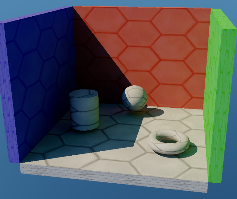
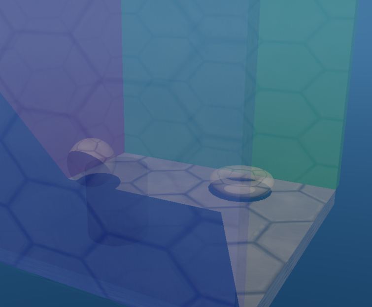
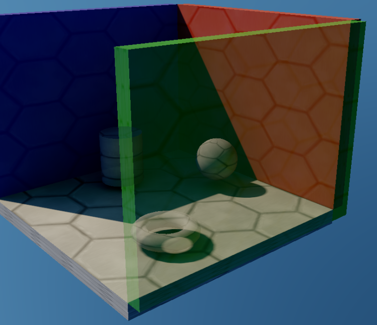
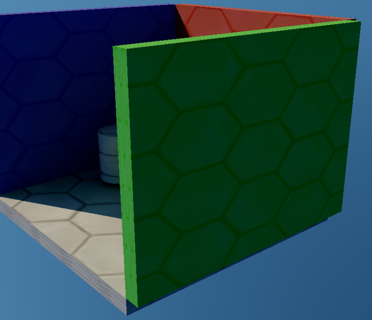
When the paper came out I read it and I was naturally interested, so I quickly hacked together a sample project using another project as a base. Unfortunately over the past 2 months there’s been holidays, the flu, and several weeks of long hours at work so that we could could finish up a major milestone. So while I’ve had time to visit my family and optimize our engine for PS4, I haven’t really had any time to come up with a proper sample app that really lets you explore the BOIT technique in a variety of scenarios. However I really hate not having source code and a working sample app to go with papers, so I’m going to release it so that others at least have something they can use for evaluating their proposed algorithm. Hopefully it’s useful, despite how bad the test scene is. Basically it’s just a simple cornell-box like scene made up of a few walls, a sphere, a cylinder, a torus, and a sky (I normally use it for GI testing), but I added the abililty to toggle through 2 alternative albedo maps: a smoke texture, and a tree texture. It doesn’t look great, but it’s enough to get a few layers of transparency with varying lighting conditions:

Scene_Normal

The sample is based on another project I’ve been working on for quite some time with my fellow graphics programmer David Neubelt, where we’ve been exploring new techniques for baking GI into lightmaps. For that project I had written a simple multithreaded ray-tracer using Embree 2.0 (which is an awesome library, and I highly recommend it), so I re-purposed it into a ground-truth renderer for this sample. You can toggle it on and off  to see what the scene would look like with perfect sorting, which is useful for evaluating the “correctness” of the BOIT algorithm. It’s very fast on my mighty 3.6GHz Core i7, but it might chug a bit for those of you running on mobile CPU’s. If that’s true I apologize, however I made sure that all of the UI and controls are decoupled from the ray-tracing framerate so that the app remains responsive.

I’d love to do a more thorough write-up that really goes into depth on the advantages and disadvantages in multiple scenarios, but I’m afraid I just don’t have the time for it at the moment. So instead I’ll just share some quick thoughts and screenshots:

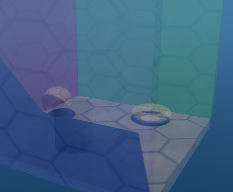
It’s pretty good for surfaces with low to medium opacity  – with the smoke texture applied, it actually achieves decent results. The biggest issues are where there’s a large difference in the lighting intensity between two overlapping surfaces, which makes sense since this also applies to improperly sorted surfaces rendered with traditional alpha blending. Top image is with Blended OIT, bottom image is ground truth:

Smoke_BOIT
Smoke_Ref

If you look at the area where the closer, brighter surface overlaps the darker surface on the cylinder you can see an example of where the results differ from the ground-truth render. Fortunately the depth weighting produces results that don’t look immediately “wrong”, which is certainly a big step up from unsorted alpha blending. Here’s another image of the test scene with default albedo maps, with an overall opacity of 0.25:

LowOpacity_BOIT
LowOpacity_Ref

The technique fails for surfaces with high opacity – one case that the algorithm has trouble with is surfaces with opacity = 1.0. Since it uses a weighted blend, the weight of the closest surface has to be incredibly high relative to any other surfaces in order for it to appear opaque. Here’s the test scene with all surfaces using an opacity of 1.0:

HiOpacity_BOIT
HiOpacity_Ref

You’ll notice in the image that the algorithm does actually work correctly with opacity = 1 if there’s no overlap of transparent surfaces, so it does hold up in that particular case. However in general this problem makes it unsuitable for materials like foliage, where large portions of of surface need to be fully opaque. Here’s the test scene using a tree texture, which illustrates the same problem:

Tree_BOIT
Tree_Ref

Like I said earlier, you really need to make the closest surface have a an extremely high weight relative to the surfaces behind it if you want it to appear opaque. One simple thing you could do is to keep track of the depth of the closest surface (say in a depth buffer), and then artificially boost the weight of surfaces if their depth matches the depth buffer weight. If you do this (and also scale your “boost” factor by opacity) you get something like this:

Tree_DBWeight

This result looks quite a bit better, although messing with the weights changes the alpha gradients which gives it a different look. This approach obviously has a lot of failure cases. Since you’re relying on depth, you could easily create discontinuities at geometry edges. You can also get situations like this, where a surface visible through a transparent portion of the closest surface doesn’t get the weight boost and remains translucent in appearance:

DBWeightFail_BOIT

DBWeight_Ref

Notice how the second tree true trunk appears to have a low opacity since it’s behind the closest surface. The other major downside is that you need to render your transparents in a depth prepass, which requires performance as well as the memory for an extra depth buffer. However you may already be doing that in order to optimize tiled forward rendering of transparents. Regardless I doubt it would be useful except in certain special-case scenarios, and it’s probably easier (and cheaper) to just stick to alpha-test or A2C for those cases.

Is it usable? – I’m not sure yet. I feel like it would take a lot of testing the wide range of transparents in our game before knowing if it’s going to work out. It’s too bad that it has failure cases, but if we’re going to be honest the bar is pretty damn low when it comes to transparents in  games. In our engine we make an attempt to sort by depth, but our artists frequently have to resort to manually setting “sort priorities” in order to prevent temporal issues from meshes constantly switching their draw order. The Blended OIT algorithm on the other hand may produce incorrect results, but those results are stable over time. However I feel the much bigger issue with traditional transparent rendering is that ordering constraints are fundamentally at odds with rendering performance. Good performance requires using instancing, reducing state changes and rendering to low-resolution render targets. All 3 of those these are incompatible with rendering based on Z order, which means living with lots of sorting issues if you want optimal performance. With that in mind it really feels like it’s hard to do worse than the current status-quo.

That’s about all I have for now. Feel free to download the demo and play around with it. If you missed it, the download link is at the top of the page. Also, please let me know if you have any thoughts or ideas regarding the practicality of the technique, since I would definitely be interested in discussing it further.


04 Feb 15:55

Dynamically Slicing Shapes

by Randy Gaul

Just this morning I finished up a small open source project, along with a huge article at gamedev.tutsplus. The open source project is an implementation of Sutherland-Hodgman clipping which can be used in many advanced shape and mesh manipulation techniques.

PolygonSplitting

Gif of the open source project in action. Slicing a quad interactively.


04 Feb 15:54

Cesium Version B25 Released

by Patrick Cozzi

Cesium version b25 is now available for download. This release includes several minor improvements and fixes as we ramp up for a big b26 release. For a full list of changes, see the change log.

This past month, we also started plugins, which are libraries that add functionality to Cesium. In addition to a few starter plugins from Analytical Graphics, Inc., Aviture contributed a plugin for navigation using the Leap Motion controller, and Geocento contributed a plugin for shape drawing and editing.

03 Feb 11:10

x86/x64 Library Numerical differences

by Ofek Shilon

There are many online sets of examples of 64 bit migration pitfalls, but I recently came across two that that appear not to be mentioned elsewhere.

First, downright compiler bugs.  We still have those and some raise their head only in 64.  (btw – my sincere apologies to Eric Brumer for venting out over him like that. He is not to blame for MS’s infuriating support policy).

Second and more importantly, different implementations of library math functions!

Here are two quick example results from VC++ 2013:

cos(0.37034934158424915),   on 32 gives 0.932200961410311 61, on 64 gives 0.93220096141031150.

cos(0.81476855148534799),   on 32 gives 0.686036806093662 47, on 64 gives 0.68603680609366235.

(on both cases, 32 was actually closer to the accurate results – but that’s probably a coincidence).

This is not the same as the compiler making different decisions on different platforms: the implementations of trigonometric functions were hand-crafted in assembly (at least in 32 bit), and each CRT version knowingly takes different code paths, based on exact platform and architecture (sometime based on run-time processor inspection).

These two examples are the bottom line of a several-day tedious debugging session.  This seemingly negligible difference manifested itself as a ~0.5% difference between results of a numerical optimization routine, in 32 and 64 bit VC++.

While not strictly a bug, this behaviour does make me uncomfortable in several aspects.

(1) Judging by some traces I compared during debugging, on ~95% of cases transcendental functions coincide exactly (to the last digit) on 32 and 64. Which makes one assume they were aiming for binary compatibility, and wonder whether the 5% difference is intentional.

(2) Stepping through the x64 implementation, it makes use of only vanilla SSE instructions, fully accessible to x86. There’s no technical reason limiting the implementations from coinciding.

(3) IEEE-754 had undergone a major overhaul in 2008, and the new version includes a much needed clause – still phrased as a recommendation. Quoting wikipedia:

…it recommends that language standards should provide a means to write reproducible programs (i.e., programs that will produce the same result in all implementations of a language), and describes what needs to be done to achieve reproducible results.

I was hoping /fp:precise would have such an effect, but apparently it doesn’t.  As far as I can say, today the only way of achieving such reproducibility is by hand crafting your own function implementations.

Or if, like me, you can live without the last digits of precision, you can just make do without them.  I now include the following code in every file that uses trig/inverse-trig functions.
[Edit: see a fix in a newer post.]

// TruncatedFuncs.h

#pragma once
#include <math.h>

inline double Truncate(double arg)
{
	__int64 &ResInt = reinterpret_cast<__int64&> (arg);
			ResInt &= 0xFFFFFFFFFFFFFFF8,  // set the final 3 bits to zero
			ResInt |= 4;   // estimate the middle of the truncated range
	double	&roundedRes = reinterpret_cast<double&> (ResInt);

	return roundedRes;
}

inline double MyCos(const double ang)
{
	return Truncate(cos(ang));
}

inline double MySin(const double ang)
{
	return Truncate(sin(ang));
}

inline double MyTan(const double ang)
{
	return Truncate(tan(ang));
}

inline double MyAcos(const double ang)
{
	return Truncate(acos(ang));
}

inline double MyAsin(const double ang)
{
	return Truncate(asin(ang));
}

inline double MyAtan2(const double y, const double x)
{
	return Truncate(atan2(y, x));
}

#define cos MyCos
#define sin MySin
#define tan MyTan
#define acos MyAcos
#define asin MyAsin
#define atan2 MyAtan2


Filed under: VC++
03 Feb 07:38

1-30-14 - Understanding ANS - 1

by cbloom
I'm trying to really understand Jarek Duda's ANS (Asymmetric Numeral System). I'm going to write a bit as I figure things out. I'll probably make some mistakes.

For reference, my links :

RealTime Data Compression Finite State Entropy - A new breed of entropy coder
Asymmetric Numeral System - Polar
arxiv [1311.2540] Asymmetric numeral systems entropy coding combining speed of Huffman coding with compression rate of arithmetic
encode.ru - Asymetric Numeral System
encode.ru - FSE
Large text benchmark - fpaqa ans
New entropy coding faster than Huffman, compression rate like arithmetic - Google Groups

I actually found Polar's page & code the easiest to follow, but it's also the least precise and the least optimized. Yann Collet's fse.c is very good but contains various optimizations that make it hard to jump into and understand exactly where those things came from. Yann's blog has some good exposition as well.

So let's back way up.

ANS adds a sequence of values into a single integer "state".

The most similar thing that we're surely all familiar with is the way that we pack integers together for IO or network transmission. eg. when you have a value that can be in [0,2) and one in [0,6) and one in [0,11) you have a range of 3*7*12 = 252 so you can fit those all in one byte, and you use packing like :


// encode : put val into state
void encode(int & state, int val, int mod)
{
    ASSERT( val >= 0 && val 
Obviously at this point we're just packing integers, there's no entropy coding, we can't do unequal probabilities. The key thing that we will keep using in ANS is in the decode - the current "state" has a whole sequence of values in it, but we can extract our current value by doing a mod at the bottom.

That is, say "mod" = 3, then this decode function can be written as a transition table :


state   next_state  val
0       0           0
1       0           1
2       0           2
3       1           0
4       1           1
5       1           2
6       2           0
...

In the terminology of ANS we can describe this as "0120120120..." or just "012" and the repeating is implied. That is, the bottom bits of "state" tell us the current symbol by looking up in that string, and then those bottom bits are removed and we can decode more symbols.

Note that encode/decode is LIFO. The integer "state" is a stack - we're pushing values into the bottom and popping them from the bottom.

This simple encode/decode is also not streaming. That is, to put an unbounded number of values into state we would need an infinite length integer. We'll get back to this some day.

02 Feb 18:26

Seven Things for February 1, 2014

by Eric

Here we go:

02 Feb 18:25

CAI: Cable And Igor's Adventures in Matrix Factorization: A Tornado Through a Parking Lot

by Igor
I was reminded of this when I watched Yi Ma's presentation at MIA2014 but it somehow felt that this is still not widely known. Trusting the underlying structure of the signal can go a long way for separating events. This is why with Cable, we played with Tianyi Zhou and Dacheng Tao's GoDec solver to produce imagery decomposition in several youtube videos and featured in CAI: Cable And Igor's Adventures in Matrix Factorization. The very important fact to retain from these experiments is that they require no knowledge of image processing. Here is an example I dug up from our archives, a tornado hitting a parking lot. Here is the initial video:


and its attendant Robust PCA decomposition.The video is decomposed in three components, a low rank one (ideally a background image in the case of rank 1) on top left portion of the screen, a sparse and noisy component (both in the bottom row).


Solvers that do similar decomposition can be found in the Advanced Matrix Factorization Page

Other videos can be found in:


Also of interest the LinkedIn Advanced Matrix Factorization Page
01 Feb 13:50

Looking For a Good Sort

by tony@overbyte.com.au (Tony Albrecht)

Vessel for PlayStation 3 has finally been submitted to Sony for approval so I have a little more time to write up some of the optimisation challenges we had to overcome during its porting process. Well, OK, I don’t really have any more time but I’ll try to write a bit more about it before wet bit rot sets in and I forget everything.

a1sx2_Thumbnail1_VesselFluid.JPG

Vessel ran predominantly on three threads; one for Physics, one for Game and one for the Render process. The Render thread translated the output from the Game thread into a command buffer that could be parsed by the SPUs and as such was pretty short - we had allocated up to 3 ms per frame for it and unfortunately, in certain places it was hitting 11ms.

Looking at a Tuner profile we found the following

FluidMeshMapStd.png

In this case, the Render thread was taking around 6ms, with half of this taken up with the generation of the quads for each of the fluid mesh maps. Of that, 1 millisecond was spent in the STL sort function. This seemed a little excessive to me, so I looked closer. The red bars in the image above correspond to the following code:

STD-code.JPG

with the following functors to do the gritty part of the sorting.


FluidFunctors.JPG

Basically, what the above code does is, for each fluid mesh map (the outer loop code isn’t shown but the first code fragment is called once per FluidMeshMap) sort the FluidVertexes by water type (lava, water, glow goo etc) and then by whether or not it is an isolated drop (both edges in the g_Mesh are equal) or if it is an edge (e1 != e2). Once that is done this information is used to populate a vertex array (via calls to SetEdge()) which is in turn eventually passed off to the GPU.

From looking at the Tuner scan we can see that the blue parts take up a fair amount of time (they correspond to PROFILE_SCOPE(sort) in the code) and correspond to the standard sort() function. The question is, can we write a better sort than std::sort?

std::sort is already highly optimised and was written by smart people that have produced a generic solution that anyone can plug into their code and use without thinking too much about it. And that is exactly why we can write a faster sort than std::sort for this case - because we know exactly what we want. We have the input and we know the output we want, all we need to do is work out the fiddly transformation bit in the middle.

The output we desire is the FluidVerts ordered by sort and then by edge/drop type. The final order should look something like this:

Output.png

I decided to base the solution loosely on the Radix sort. We do a first pass over the data to be sorted and count up how many of each fluid ‘sort’ there is. This is then effectively a histogram of the different fluid types - we now know how many of each type there is and we can set up a destination array that is the size of the sorted elements and we can calculate where in that contiguous array the ‘sorts’ of fluid should go.

Our second pass steps through the source array and places the FluidVertex into the correct bucket (based on fluid ‘sort’), but adds it to the beginning of the bucket if it is an edge and at the end if it is a drop. And that’s it. Done. Two passes. A super fast, super simple sort that does just what we need.

“So, how much faster is it then?” I hear you ask.

“About five times faster.” I would respond. This sort runs in about .25ms compared to the original 1ms but it also has the added benefit of moving the FluidVertex data into contiguous sorted arrays (the original just produced an index map that could be used to traverse the original array (vSorted)). This is good because we can then easily optimise the second part of the FluidMeshMap loop which copies the verts to a vertex buffer for rendering and also modifies the edges via calls to SetEdge() (for those that are interested, the SetEdge() function does some simple arithmetic and inconveniently calls Atan2() to set up the angle of the edge for the GPU to use). This contiguous data means fewer cache misses, but on PS3 it also means that we can easily pass it off to the SPUs to do the transform and copy for us while we process the next FluidMeshMap on the PPU. Nice huh?

The result is that the BuildFluidMeshmap section is reduced from 2.25ms down to 0.24ms - a saving of 2ms

FluidMeshMapSimple.png

The key message to take away from this is that generic implementations of algorithms are great for getting your code up and running quickly, but don’t expect them to be lightning fast in all cases. Think about what you are doing, reduce you problem to the simplest inputs and outputs and then build a simple transformation that does just that. It will make you feel good on the inside. Simplicity is its own reward.

(For anyone interested in more sorting goodness, check out an old blog post of mine A Questions of Sorts.) 


31 Jan 08:32

A better Sketchfab is coming

image

When Sketchfab was first started, it was really just a technology; a viewer that allowed anyone to display 3D files in the browser. Over time, it became clear to us that what we were actually building was something much greater - it was turning into a real community. 

With that in mind, the team has been hard at work building V2 of Sketchfab. The site in its current form has been a great starting point - easy uploading, staff picked galleries to show off the amazing work being created, and smart tools to ease your workflow. But we know there’s a lot of room for improvement, and want to make it easier for the community to connect with each other, and ultimately help you make your 3D content social. Thats been the inspiration behind V2, and we think you’re going to really love the new design and features we have in store for you. 

To kick things off, what you see above will be our new logo. You’ve probably seen it popping up already on a few places like our Photoshop integration, our Google+ page or our new meetup group. It’s a small taste of whats to come in the next few months… stay tuned :) 

ps: quick tip, come to our 1st NYC meetup, Tuesday February 11th, if you want a sneak-peak!

image


PoustEx from BaloOm on Sketchfab.

31 Jan 08:31

GLSL multidimensional array... madness?

Multidimensional arrays are added to GLSL via either GL_ARB_arrays_of_arrays extension or GLSL 4.30. I've had a couple people tell me that the multidimensional array syntax is either wrong or just plain crazy. When viewed from the proper angle, it should actually be perfectly logical to any C / C++ programmer. I'd like to clear up a bit of the confusion.

Staring with the easy syntax, the following does what you expect:

    vec4 a[2][3][4];

If a is inside a uniform block, the memory layout would be the same as in C. cdecl would call this, "declare a as array 2 of array 3 of array 4 of vec4".

Using GLSL constructor syntax, the array can also be initialized:

    vec4 a[2][3][4] = vec4[][][](vec4[][](vec4[](vec4( 1), vec4( 2), vec4( 3), vec4( 4)),
                                          vec4[](vec4( 5), vec4( 6), vec4( 7), vec4( 8)),
                                          vec4[](vec4( 9), vec4(10), vec4(11), vec4(12))),
                                 vec4[][](vec4[](vec4(13), vec4(14), vec4(15), vec4(16)),
                                          vec4[](vec4(17), vec4(18), vec4(19), vec4(20)),
                                          vec4[](vec4(21), vec4(22), vec4(23), vec4(24))));

If that makes your eyes bleed, GL_ARB_shading_language_420pack and GLSL 4.20 add the ability to use C-style array and structure initializers. In that model, a can be initialized to the same values by:

    vec4 a[2][3][4] = {
        {
            { vec4( 1), vec4( 2), vec4( 3), vec4( 4) },
            { vec4( 5), vec4( 6), vec4( 7), vec4( 8) },
            { vec4( 9), vec4(10), vec4(11), vec4(12) }
        },
        {
            { vec4(13), vec4(14), vec4(15), vec4(16) },
            { vec4(17), vec4(18), vec4(19), vec4(20) },
            { vec4(21), vec4(22), vec4(23), vec4(24) }
        }
    };

Functions can be declared that take multidimensional arrays as parameters. In the prototype, the name of the parameter can be present, or it can be omitted.

    void function_a(float a[4][5][6]);
    void function_b(float  [4][5][6]);

Other than the GLSL constructor syntax, there hasn't been any madness yet. However, recall that array sizes can be associated with the variable name or with the type. The prototype for function_a associates the size with the variable name, and the prototype for function_b associates the size with the type. Like GLSL constructor syntax, this has existed since GLSL 1.20.

Associating the array size with just the type, we can declare a (from above) as:

    vec4[2][3][4] a;

With multidimensional arrays, the sizes can be split among the two, and this is where it gets weird. We can also declare a as:

    vec4[3][4] a[2];

This declaration has the same layout as the previous two forms. This is usually where people say, "It's bigger on the inside!" Recall the cdecl description, "declare a as array 2 of array 3 of array 4 of vec4". If we add some parenthesis, "declare a as array 2 of (array 3 of array 4 of vec4)", and things seem a bit more clear.

GLSL ended up with this syntax for two reasons, and seeing those reasons should illuminate things. Without GL_ARB_arrays_of_arrays or GLSL 4.30, there are no multidimensional arrays, but the same affect can be achieved, very inconveniently, using structures containing arrays. In GLSL 4.20 and earlier, we could also declare a as:

    struct S1 {
        float a[4];
    };

    struct S2 {
        S1 a[3];
    };

    S2 a[2];

I'll spare you having to see GLSL constructor initializer for that mess. Note that we still end up with a[2] at the end.

Using typedef in C, we could also achieve the same result using:

    typedef float T[3][4];

    T a[2];

Again, we end up with a[2]. If cdecl could handle this (it doesn't grok typedef), it would say "declare a as array 2 of T", and "typedef T as array 3 of array 4 of float". We could substitue the description of T and, with parenthesis, get "declare a as array 2 of (array 3 of array 4 of float)".

Where this starts to present pain is that function_c has the same parameter type as function_a and function_b, but function_d does not.

    void function_c(float[5][6] a[4]);
    void function_d(float[5][6]  [4]);

However, the layout of parameter for function_e is the same as function_a and function_b, even though the actual type is different.

    struct S3 {
        float a[6];
    };

    struct S4 {
        S3 a[5];
    };

    void function_e(S4 [4]);

I think if we had it to do all over again, we may have disallowed the split syntax. That would remove the more annoying pitfalls and the confusion, but it would also remove some functionality. Most of the problems associated with the split are caught at compile-time, but some are not. The two obvious problems that remain are transposing array indices and incorrectly calculated uniform block layouts.

    layout(std140) uniform U {
        float [1][2][3] x;
        float y[1][2][3];
        float [1][2] z[3];
    };

In this example x and y have the same memory organization, but z does not. I wouldn't want to try to debug that problem.

31 Jan 08:30

GPU Pro 5 – Quaternions Revisited

by Peter Sikachev
Our GPU Pro 5 chapter describes experience of migrating normal mapping, skinning, instancing, morph targets, non-uniform scale and other features from matrix representation to quaternions. It is based on the practical implementation in the Skyforge next-gen MMORPG title. In particular, we claim to develop a novel seamless method for vertex quaternion alignment with zero overhead for correctly UV-mapped polygonal meshes.

Most of modern rendering engines take advantage of per-pixel shading techniques such as normal mapping. In order to have a normal map properly mapped to the mesh surface, one should define a tangent space at each its vertex, also known as tangent-bitangent-normal (TBN). However, using TBN leads to several performance/memory negative effects: it needs at least 7 bytes per vertex, consumes a lot of shader interpolators, requires re-orthogonalization after interpolation etc. Therefore, certain rendering engines try to replace them. One common choice is using quaternions instead.

Quaternions themselves have a number of cases to take care of: they should be aligned to be interpolated properly, the skinning becomes tricky etc. In this article we present a thorough description of quaternions’ tricks and pitfalls in a rendering engine, based on our experience: starting from data export and compression to such advanced topics as skinning, morph targets etc. We back up our description with comprehensive listings in C++/HLSL/pseudocode, including quaternion alignment algorithm, developed by authors, which eliminates the normal seams on parameterized surfaces.

Proposed methods and techniques have been implemented in the next-gen MMORPG, developed by Mail.Ru Group.


Incorrectly interpolated quaternions (left),
correctly interpolated quaternions after alignment (right).
Image courtesy of Mail.Ru Group.
30 Jan 12:45

Coherent Noise for Non-Photorealistic Rendering
Coherent Noise for Non-Photorealistic Rendering

Michael Kass, Davide Pesare
July 2011

A wide variety of non-photorealistic rendering techniques make use of random variation in the placement or appearance of primitives. In order to avoid the "shower-door" effect, this random variation should move with the objects in the scene. Here we present coherent noise tailored to this purpose. We compute the coherent ... [more]

Available in the Proceedings of SIGGRAPH 2011


Site last built: Tue Jan 28 09:31:10 2014

This post has been generated by Page2RSS
30 Jan 09:18

Visual Studio 2013 Update 1

by Chuck Walbourn - MSFT
pAn update to Visual Studio 2013 is now available for a href="http://go.microsoft.com/fwlink/?LinkId=301714"download/a./p pFor more details see a href="http://blogs.msdn.com/b/visualstudio/archive/2014/01/21/update-1-for-visual-studio-2013.aspx"Visual Studio Team Blog/a, a href="http://blogs.msdn.com/b/bharry/archive/2014/01/20/vs-2013-1-update-1-is-available.aspx"Brian Harryrsquo;s blog/a, and a href="http://blogs.msdn.com/b/somasegar/archive/2014/01/20/visual-studio-2013-update-1.aspx"Somasegarrsquo;s blog/a./p pOfficial KB article a href="http://support.microsoft.com/kb/2911573"2911573/a/p pstrongNote:/strong The version of compiler (18.00.21005.1) and C/C++ Runtime (12.0.21005.1) are the same ones that shipped with VS 2013 RTM. There is an a href="http://go.microsoft.com/fwlink/?LinkId=386813"updated Remote Debugging Tools package/a for VS 2013 Update 1./p pstrongRelated:/strong a href="http://blogs.msdn.com/b/chuckw/archive/2013/10/18/visual-studio-2013-and-windows-8-1-sdk-rtm-are-now-available.aspx"Visual Studio 2013 RTM/a, a href="http://blogs.msdn.com/b/chuckw/archive/2014/05/12/visual-studio-2013-update-2.aspx"VS 2013 Update 2/a, a href="http://blogs.msdn.com/b/chuckw/archive/2014/08/05/visual-studio-2013-update-3.aspx"VS 2013 Update 3/a, a href="http://blogs.msdn.com/b/chuckw/archive/2014/11/24/visual-studio-2013-update-4.aspx"VS 2013 Update 4/a/pdiv style="clear:both;"/divimg src="http://blogs.msdn.com/aggbug.aspx?PostID=10495482" width="1" height="1"
30 Jan 08:12

Now live on Steam Greenlight!

by Sophie Schiaratura

We’ve gone ahead and posted Algo-Bot on Steam.

By voting for Algo-Bot on Greenlight, you increase the chances that Valve will distribute the game through Steam. This is pretty important for improving the game’s visibility, and provides a secure, reliable way of distributing the game files automatically to our users.


greenlight_algo-bot_455


Greenlight is extremely competitive, so if you’re excited about Algo-Bot, share the Greenlight link with your friends and vote “YES”! Your move!

Thank you!

30 Jan 08:11

mitmproxy and pathod 0.10

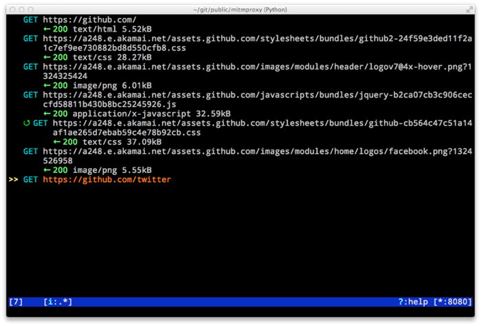
mitmproxy and pathod 0.10

29 January 2014

I've just released v0.10 of both mitmproxy and pathod. This is chiefly a bugfix release, with a few nice additional features to sweeten the pot.

Perhaps the most visible change has been a huge improvement in the recommended method for installing the mitmproxy certificates. Certs are now served straight from the web application hosted in mitmproxy, which means that in most cases cert installation is as simple as typing the mitmproxy URL into the devce driver. See the docs for more.

In other, minor news - I see that the mitmproxy project has just passed 2000 stars on GitHub. Between PyPi and the files we serve from mitmproxy.org, the project has also seen nearly 100k downloads in the last year (after removing obvious bots). I know, I know - figures like these don't mean much, but it's still nice to see that people are using and enjoying mitmproxy.

CHANGELOG

  • Support for multiple scripts and multiple script arguments
  • Easy certificate install through the in-proxy web app, which is now enabled by default
  • Forward proxy mode, that forwards proxy requests to an upstream HTTP server
  • Reverse proxy now works with SSL
  • Search within a request/response using the "/" and "n" shortcut keys
  • A view that beatifies CSS files if cssutils is available
  • Many bug fix, documentation improvements, and more.
29 Jan 07:39

Let the revolution begin: key 3D printing patent expires today

Today may be a milestone in the 3D printing revolution: one of the key 3D printing patents related to Selective Laser Sintering (SLS) technology expires today. The patent under question is that of Carl R. Deckard which was filed on May 31 1994 and issued on 28 January 1997.

This article Let the revolution begin: key 3D printing patent expires today is first published at 3ders.org.

29 Jan 07:38

CMake 2.8.12.2 available for download

by Robert Maynard

Some problems were reported with the 2.8.12 release. Thanks to the work of Brad King, Robert Maynard, Rolf Eike Beer, Ruslan Baratov, and Ted Kremenek those problems have been fixed. We've prepared a 2.8.12.2 bug fix release to address those issues.

Some of the notable changes in this patch release are:

  • XCode: Fix compiler line matching for XCode 5.1
  • Visual Studio: Convert include path to backslashes for Visual Studio 2010 and newer
  • FindOpenMP: Support compilers that do not need any special flags
 
The complete list of changes in 2.8.12.2 can be found at:
29 Jan 07:38

Jolt Awards: Coding Tools

The best IDEs and coding tools of the past 12 months
29 Jan 07:35

The Role of Algorithms in Data Visualization

by Enrico
It’s somewhat surprising to me to notice how little we discuss about the more technical side of data visualization. I use to say that visualization is something that “happens in your head” to emphasize the role of perception and cognition and to explain why it is so hard to evaluate visualization. Yet, visualization happens a […]
29 Jan 07:34

Leveling Lakes

by Miguel Cepero
This post will advance the water saga.

You may want to check out the previous post about water. It ended up producing a 2D map of booleans, where true meant there was water in that location of the map. That was great, but we still had a nasty problem ahead. We needed to level the lakes.

It will be easier if we look at some pictures. Imagine this is the tile we need to compute. Initially it is just the terrain height and the sea map (in this case using a sea-level value):


And here you can see the lake and river location phase from the earlier post in pretty pink:


As you can see in the zoomed portion, these lakes often span over very irregular terrain. We knew the shoreline points for the same lake were at similar height. Figuring out the water level from A to B was the problem. We know A-B should be as flat as possible and the same applies to A and any other point in the shoreline. That's a lot of potential points.

If we had all the time in the world, we could try discovering individual lakes in one phase and then do some sort of iterative leveling by relaxation and or filtering. We had only a fraction of a second for this so we knew it had to be hacked.

We tried many different things. (When I say "we", it is not modesty plural. Michael Coates who recently joined Voxel Farm got to implement these desperate things we tried.) Most had to do with rasterization and interpolation, first from shore to shore, then we got looking into water height derivatives. Nothing really worked.

As a last recourse attempt, we tried an approach that involved a Quadtree. The idea was to encode the water bodies in a Quadtree and apply the same leveling algorithms we knew would be too slow if we were operating in individual water samples.

The shorelines produced a lot of small quads, but as we moved inside the lake we started getting larger quads.


We could see that the larger a patch, the more "detached" it was from the shore. That we liked. We could raise or sink those points much more to achieve the level we needed.

Once the water height of the larger patches is decided, we rasterize them into the water heightmap. This is a simple, fast bi-linear interpolation over the quad. Then we do the same for the smaller quads. There is a reason why you need to process all quads of a given size before processing the next level of smaller patches: You need to make sure the small quads match the interpolation values along the edges they share with a larger quad.

This overall process is quite fast. Here is a rendering of the new found water volumes. It is a bit exaggerated, but hopefully you get the idea:


We still need to work out on some of the heuristics, but it looks we are pretty much on our way.

If there is any lesson to be drawn from this, it would be when in despair, apply a Quadtree and everything will be alright.
28 Jan 13:02

(Pre)release IRHydra 2.0

by Vyacheslav Egorov
26 Jan 16:51

Akira inspired Zelda

by Nic
26 Jan 16:50

Photosynth 2 launch!

by Henri

Happy new year 2014!

This is a short post in case you’ve missed the launch of Photosynth2. I’m glad to be able to break the silence and to show some nice stuff again :) . I’ve developed the WebGL viewer used to display ps2 synths and I’ve been busy capturing tons of ps2′s (I still have a lot of datasets waiting to be uploaded :) ).

If you are using a modern browser you should be able to see this ps2 with the WebGL viewer:

Otherwise we are also generating an mp4 fallback:

poster="https://ssl-cdn.ps1.photosynth.net/media/19d5cf2b-77ed-439f-ac21-d3046320384c/packet/thumbs/default/poster.jpg">

In case you are wondering what’s new compared to photosynth1, I’ve created this video showing the benefit of a ‘good’ geometry (ps2) for image-based rendering instead of using only a dominant plane (ps1):

Photosynth 1 is allowing unstructured capture and thus the navigation is very difficult. In Photosynth 2 we are constraining the user to capture images along a single path (1D manifold) and thus the navigation is very simple (and touch friendly :-) ). Photosynth 2 introduces 4 different topology (camera motions):

Spin:

Panorama:

Walk:

Wall:

BTW if you type: “The answer to life, the universe and everything”, on the view page of a synth a magic menu will appear with lot of options so that you can tweak your viewer. You will need to refresh the view page to apply most options and the changes are permanent (store in localStorage).


‘m’ and ‘c’ are also two other shorcuts that you should try…

I should have another post very soon. Stay tuned!

Share

26 Jan 16:50

Epic software rant

by Mark Liberman

From Dave Noon, "Christ, I hate Blackboard", Lawyers, Guns & Money 1/24/2014:

Hundreds of years from now, after disease and fire and famine have thinned the human herd to a shrunken patchwork of sagging, skeletal bands of jagged, half-mad wraiths — when the parched soil chokes forth desiccated roots and the air is a toxic brume slumping down on the arched, knotted backs of the still-barely-living — a remote spur of humanity will somehow recover the capacity to speak, an ability long since abandoned by their ancestors, who were mute-struck with the unfathomable despair of those cursed to watch everything they love die. After generations of dry-throated croaking and lung-starched wheezing, their tongues swollen with thirst and punctured with abscesses that never heal, these distant people will bring forth a new language to survey the boundaries of their pain. [...]

On the outskirts of this new language, lurking on its crimsoned frontier, will lie words that will themselves have been cast into exile – foul offgassings within a lexicon that itself stands as a towering monument to the boundlessly obscene, words that will curve backward and devour themselves, each one an afflicted universe in the process of total collapse, words that exist for microseconds before streaking, unremembered and unmourned, into the void.  

These are the words, if I could shit them into being, that I would use to catalogue the depth of my loathing for Blackboard.

You should definitely read the whole thing.

Why are certain types of software systems so reliably bad? In my understanding, it's a combination of the process of specification and implementation, the (mis-)education and general outlook of the designers and implementers, and the characteristics that the people in charge are actually trying to optimize.

We've commented on some of these issues from time to time in the past, e.g. "If you can answer this, you are not paying attention", 7/10/2006, or "When bad interaction happens to good people", 8/15/2007. (That last post dealt with a system for which I wrote a tongue-in-cheek-but-serious Users Guide, "The Legend of FacilityFocus". The software has since been improved in ways that make it substantially easier to navigate, though there are still difficulties due to things like systematic differences between floor numbering in the master database and floor numbering as marked on the building signage…)

I tried using Blackboard once, many years ago when my institution first switched to it. I gave up for two reasons: it was an order of magnitude harder than just putting stuff up on the web; and all the stuff I painfully entered in it vanished from one year to the next, on purpose but without warning.  Penn has now switched to Canvas, which I haven't yet tried.

I do use Piazza, and generally find it well designed and helpful — I suspect that this is because it came out of a different sort of development process.

26 Jan 16:48

512 and counting

by Eric

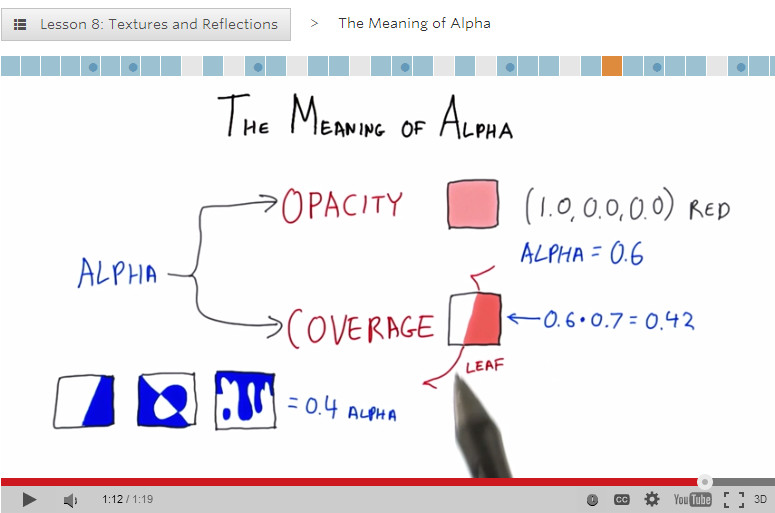
I noticed I reached a milestone number of postings today, 512 answers posted to the online Intro to 3D Graphics course. Admittedly, some are replies to questions such as “how is your voice so dull?” However, most of the questions are ones that I can chew into. For example, I enjoyed answering this one today, about how diffuse surfaces work. I then start to ramble on about area light sources and how they work, which I think is a really worthwhile way to think about radiance and what’s happening at a pixel. I also like this recent one, about z-fighting, as I talk about the giant headache (and a common solution) that occurs in ray tracing when two transparent materials touch each other.

So the takeaway is that if you ever want to ask me a question and I’m not replying to email, act like you’re a student, find a relevant lesson, and post a question there. Honestly, I’m thoroughly enjoying answering questions on these forums; I get to help people, and for the most part the questions are ones I can actually answer, which is always a nice feeling. Sometimes others will give even better answers and I get to learn something. So go ahead, find some dumb answer of mine and give a better one.

By the way, I finally annotated the syllabus for the class. Now it’s possible to cherry-pick lessons; in particularly, I mark all lessons that are specifically about three.js syntax and methodology if you already know graphics.

alpha

25 Jan 13:00

Why Do Quaternions Double-Cover?

by Nathan Reed

Quaternions are pretty well-known to graphics programmers at this point, but even though we can use them for rotating our objects and cameras, they’re still pretty mysterious. Why are they 4D instead of 3D? Why do the formulas for constructing them have factors like \(\cos\theta/2\) instead of just \(\cos\theta\)? And why do they have the “double-cover” property, where there are two different quaternions (negatives of each other) that represent the same 3D rotation?

These properties need not be inexplicable teachings from on high—and you don’t have to go get a degree in group theory to comprehend them, either. There are actually quite understandable reasons for quaternions to be so weird, and I’m going to have a go at explaining them.


Numbers That Rotate

Quaternions are basically complex numbers that have eaten a super mushroom and become twice as big, so it’s helpful to understand complex numbers before going on. The main property of complex numbers that’s important here is how they represent rotations in 2D. Unfortunately, if you grew up in the USA you were probably never introduced to this in school—you probably learned all about how \(i^2 = -1\), but nothing about how complex numbers represent rotations. Steven Wittens’ How to Fold a Julia Fractal is a neat article with interactive diagrams that explain complex numbers from the geometric perspective.

The main fact we need here is just this: multiplying by a unit complex number is equivalent to rotating in 2D space: \[ (\cos\theta + i \sin\theta) (x + iy) = (x\cos\theta – y\sin\theta) + i(x\sin\theta + y\cos\theta) \] Here, I’m multiplying two complex numbers, but the one on the right, \(x + iy\), I’m thinking of as just a point in 2D space; the one on the left, \(\cos\theta + i\sin\theta\), I’m thinking of as a transformation—namely a rotation by \(\theta\). And as you can see, when I multiply them, the result is the point \((x, y)\) rotated by \(\theta\).

In particular, if I set \(\theta = \pi/2\), then the number on the left just reduces to \(i\). So multiplying by \(i\) does a 90-degree rotation: \[ (i) (x + iy) = -y + ix \]

Rotate All The Dimensions!

OK, complex numbers are cute and all, but we really want to rotate in 3D. So how can we do that?

First of all, we can’t actually create a complex-number-like algebra that works in 3D. What happens if we try? In 2D, we used real numbers for the x-axis, and imaginary numbers (proportional to \(i\)) for the y-axis. Let’s make up a brand-new imaginary unit, \(j\), which (we declare by fiat) isn’t equal to any of the existing complex numbers. This unit will represent the z-axis, so we can represent a point in 3D like \(x + iy + jz\). So far so good. But now let’s try rotating this point, by multiplying it by \(i\): \[ (i)(x + iy + jz) = -y + ix + (ij)z \] Whoops! What’s that \(ij\) thing? It can’t be reduced to a real number, or to anything proportional to \(i\) or \(j\). So it can’t represent a point in our 3D space. It’s an extra dimension! We tried to make an algebra in 3D, but found ourselves in 4D instead. If we define \(k \equiv ij\), we’ve just invented quaternions. (Well, almost. We also have to declare that \(i\) and \(j\) anticommute, i.e. that \(ij = -ji\).)

The takeaway here is that due to different imaginary units multiplying with each other, you can only create complex-like algebras in power-of-two-dimensional spaces. But let’s not give up yet. After all, 3D space is embedded in 4D space, so can’t we get 3D rotations by doing 4D rotations that are restricted to the 3D subspace?

Quaternions do represent rotations in 4D, in a similar manner to how complex numbers represent rotations in 2D. If I think of an arbitrary quaternion as a point in 4D space, and then multiply it (on the left) by \(i\), I get: \[ (i)(w + ix + jy + kz) = -x + iw – jz + ky \] Let’s look at what happened here. The \((w, x)\) components of the point became \((-x, w)\), which is a 90-degree rotation in the \(wx\) plane. Simultaneously, the \((y, z)\) components became \((-z, y)\), which is another 90-degree rotation, in the \(yz\) plane!

In general—in any number of dimensions—rotation takes place in a 2D plane. In 2D space, there’s just the one plane, so there’s just one dimension of rotation. In 3D, we talk about rotating about an axis, but we really mean rotating in a plane perpendicular to that axis. In 4D, there are enough dimensions that it’s possible to rotate in two independent planes at once—here, the \(wx\) and \(yz\) planes. The planes have no axes in common; they intersect only at a single point, which is the center of rotation, so both rotations can take place without disturbing each other (not possible in 3D, where two planes always intersect in a line).

It turns out that multiplying by a quaternion always rotates in two independent planes at once, by the same angle:

  • \(i\) rotates in the \(wx\) and \(yz\) planes.
  • \(j\) rotates in the \(wy\) and \(zx\) planes.
  • \(k\) rotates in the \(wz\) and \(xy\) planes.

Other (non-axis-aligned) quaternions rotate in other (non-axis-aligned) pairs of planes, or by other angles (not 90 degrees). Moreover, one of the two planes always includes the \(w\) axis—i.e., the axis of real numbers. This isn’t what we want for 3D rotation; we need to be able to rotate in just one plane, and we need to be able to choose any plane in the \(xyz\) subspace.

So far, we’ve multiplied a point on the left by \(i\). But quaternion multiplication isn’t commutative, so what happens when we multiply on the right? \[ (w + ix + jy + kz)(i) = -x + iw + jz – ky \] What happened here? The \((w, x)\) components went to \((-x, w)\), which is the same as before. However, the \((y, z)\) components went to \((z, -y)\), which is different. They still rotated 90 degrees, but in the opposite direction! It turns out that in general, swapping the order will reverse the direction of rotation in one of the two planes—namely, the one that doesn’t contain the \(w\) axis.

We can see now how to get our rotations to be restricted to just one plane in 4D. If we multiply on both the left and the right, the rotation whose sign changed will cancel out, and the other rotation will be done twice! \[ (i)(w + ix + jy + kz)(i) = -w – ix + jy + kz \] Just as expected, the \((w, x)\) components became \((-w, -x)\), i.e. a 180-degree rotation; the \((y, z)\) components were left unchanged.

We’re almost there. We actually don’t want to rotate the plane that includes the \(w\) axis; we’d rather it stayed fixed and the other one survived. We can do this by just inverting the quaternion on the right: \[ (i)(w + ix + jy + kz)(i^{-1}) = (i)(w + ix + jy + kz)(-i) = w + ix – jy – kz \] The inversion, as you’d expect, flips the direction of rotation in both planes—so the end result here is that the \(wx\) rotation is canceled out and the \(yz\) rotation is done twice.

So, Why Do Quaternions Double-Cover?

First of all, we can see now why quaternions have half-angles in their formulas, like \(\cos\theta/2\). To get a rotation that only affects a single plane in 4D, we have to apply the quaternion twice, multiplying on both the left and (with its inverse) on the right. The rotation we want gets done twice (and the one we don’t want gets canceled out), so we have to halve the angle going in to make up for it.

Because of that, a quaternion that rotates 180 degrees in 4D ends up rotating 360 degrees, thus doing nothing, when we apply it twice to restrict it to 3D. People say sometimes that quaternions have “720 degrees” of rotation internally. That’s one way to think about it; another way is that quaternions just have the usual 360 degrees of rotation, but you always have to apply them twice.

So if you take a quaternion and rotate it 180 degrees in 4D (i.e. negate it), it’s a different quaternion—but when applied-twice, it totals an extra 360 degrees and therefore has the same effect as the original. You can also see it algebraically: \(qpq^{-1} = (-q)p(-q)^{-1}\) since the two minus signs cancel out.

Postscript: Arbitrary 4D Rotations

You might be wondering at this point how quaternions can represent arbitrary 4D rotations. As mentioned before, a single quaternion always rotates in two independent planes by the same angle, and one of those planes always includes the \(w\) axis. So how can we rotate in two independent planes by different angles, or in planes that don’t include the \(w\) axis?

It turns out you can do this by applying two distinct quaternions, one on the left and one on the right, like \(apb\) where \(p\) is the point being rotated. For 3D rotations, \(b = a^{-1}\); for arbitrary 4D rotations, \(a\) and \(b\) don’t have any particular relationship. But the idea is generally the same: choose \(a\) and \(b\) so that two combine to cancel out the planes you don’t want and keep the ones you do want.

Why do you need this odd double-quaternion construction for arbitrary 4D rotations, while in 2D a single complex number does the job? It comes down to degrees of freedom. In 2D, there’s one dimension of rotation, and one dimension of unit complex numbers. In 4D, there are six dimensions of rotation (count ’em: \(wx, wy, wz, xy, xz, yz\)) but only three dimensions of unit quaternions—so you need to double down on quaternions to have enough degrees of freedom for a 4D rotation.

Further Reading