Nosimpler

Are emergent properties really for losers? Why are architectures important? What are “mirror neuron ensembles” anyway? My last post presented an idiosyncratic distillation of the Big Ideas in Cognitive Neuroscience symposium, presented by six speakers at the 2017 CNS meeting. Here I’ll briefly explain what I meant in the bullet points. In some cases I didn't quite understand what the speaker meant so I used outside sources. At the end is a bonus reading list.

The first two speakers made an especially fun pair on the topic of memory: they held opposing views on the “engram”, the physical manifestation of a memory in the brain.¹ They also disagreed on most everything else.


1. Charles Randy Gallistel (Rutgers University) – What Memory Must Look Like

Gallistel is convinced that Most Neuroscientists Are Wrong About the Brain. This subtly bizarre essay in Nautilus (which was widely scorned on Twitter) succinctly summarized the major points of his talk. You and I may think the brain-as-computer metaphor has outlived its usefulness, but Gallistel says that “Computation in the brain must resemble computation in a computer.” 

• The brain is an information processing device in the sense of Shannon information theory.

Shannon information is a set of possible messages encoded as bit patterns and sent over a noisy channel to a recipient that will hopefully decode the message with minimal error. In this purely mathematical theory, the semantic content (meaning) of a message is irrelevant. The brain stores numbers and that's that.

• Memories (“engrams”) are not stored at synapses.

Instead, engrams reside in molecules inside cells. The brain “encodes information into molecules inside neurons and reads out that information for use in computational operations.” A 2014 paper on conditioned responses in cerebellar Purkinje cells was instrumental in overturning synaptic plasticity (strengthening or weakening of synaptic connections) as the central mechanism for learning and memory, according to Gallistel.² Most other scientists do not share this view.³

• The engram is inter-spike interval.

Spike train solutions based on rate coding are wrong. Meaning, the code is not conveyed by the firing rate of neurons. Instead, numbers are conveyed to engrams via a combinatorial interspike interval code. Engrams then reside in cell-intrinsic molecular structures. In the end, memory must look like the DNA code.

• Emergent properties are for losers.

“Emergent property” is a code word for “we don't know.”



2. Tomás Ryan (@TJRyan_77) – Information Storage in Memory Engrams

Ryan began by acknowledging that he had tremendous respect for Gallistal's speech — which was in turn powerful, illuminating, very categorical, polarizing, and rigid. But wrong. Oh so very wrong. Memory is not essentially molecular, we should not approach memory and the brain from a design perspective, and information storage need not mimic a computer.

• The brain does not use Shannon information.

More precisely, “the kind of information the brain uses may be very different from Shannon information.” Why is that? Brains evolved, in kludgy ways that don't resemble a computer. The information used by the brain may be encoded without having to reduce it to Shannon form, and may not be quantifiable as units.

• Memories (“engrams”) are not stored at synapses.

Memory is not stored by changes in synaptic weights, Ryan and Gallistel agree on this. The dominant view has been falsified by a number of studies — including one by Ryan and colleagues that used engram labeling. Specific “engram cells” can be labeled during learning using optogenetic techniques, and later stimulated to induce the recall of specific memories. These memories can be reactivated even after protein synthesis inhibitors have (1) induced amnesia, and (2) prevented the usual memory consolidation-related changes in synaptic strength.

• We learn entirely through spike trains.

Spike trains are necessary but not sufficient to explain how information is coded in the brain. On the other hand, instincts are transmitted genetically and are not learned via spike trains.

• The engram is an emergent property.

And fitting with all of the above, “the engram is an emergent property mediated through synaptic connections” (not through synaptic weights). Stable connectivity is what stores information, not molecules.


Angela Friederici (Max Planck Institute for Human Cognitive and Brain Sciences) – Structure and Dynamics of the Language Network

Following on the heels of the rodent engram crowd, Friederici pointed out the obvious limitations of studying language as a human trait.

• Language is genetically predetermined.

The human ability to acquire language is based on a genetically predetermined structural neural network. Although the degree of innateness has been disputed, a bias or propensity of brain development towards particular modes of information processing is less controversial. According to Friederici, language capacity is rooted in “merge”, a specific computation that binds words together to form phrases and sentences.

• The “merge” computation is localized in BA 44.

This wasn't one of my original bullet points, but I found this statement rather surprising and unbelievable. It implies that our capacity for language is located in the anterior ventral portion of Brodmann's area 44 in the left hemisphere (the tiny red area in the PHRASE > LIST panel below).



The problem is that acute stroke patients with dysfunctional tissue in left BA 44 do not have impaired syntax. Instead, they have difficulty with phonological short-term memory (keeping strings of digits in mind, like remembering a phone number).

• There is something called mirror neural ensembles.

I'll just have to leave this slide here, since I really didn't understand it, even on the second viewing.



“This is a poor hypothesis,” she said.


Jean-Rémi King (@jrking0) – Parsing Human Minds

King's expertise is in visual processing (not language), but his talk drew parallels between vision and speech comprehension. A key goal in both domains is to identify the algorithm (sequence of operations) that translates input into meaning.

• Recursion is big. 

Despite these commonalities, the structure of language presents the unique challenge of nesting (or recursion): each constituent in a sentence can be made of subconstituents of the same nature, which can result in ambiguity.

• Architectures are important. 

Decoding aspects of a sensory stimulus using MEG and machine learning is lovely, but it doesn't tell you the algorithm. What is the computational architecture? Is it sustained or feedforward or recurrent?

Each architecture could be compatible with a pattern of brain activity at different time points. But do the classifiers at different time points generalize to other time points? This can be determined by a temporal generalization analysis, which “reveals a repertoire of canonical brain dynamics.”


Danielle Bassett (@DaniSBassett) – A Network Neuroscience of Human Learning: Potential to Inform Quantitative Theories of Brain and Behavior

Bassett previewed an arc of exciting ideas where we've shown progress, followed by frustrations and failures, which may ultimately provide an opening for the really Big Ideas. Her focus is on learning from a network perspective, which means patterns of connectivity in the whole brain. What is the underlying network architecture that facilitates the spatial distributed effects?



What is the relationship between these two notions of modularity?
[I ask this as an honest question.]

Major challenges remain, of course.

• Build a bridge from networks to models of behavior.

• Use generative models to construct theories. 

John Krakauer (@blamlab) – Big Ideas in Cognitive Neuroscience: Action

Krakauer mentioned the Big Questions in Neuroscience symposium at the 2016 SFN meeting, which motivated the CNS symposium as well as a splashy critical paper in Neuron. He raised an interesting point about how the term “connectivity” has different meanings, i.e. the type of embedded connectivity that stores information (engrams) vs. the type of correlational connectivity when modules combine with each other to produce behavior. [BTW, is everyone here using “modules” in the same way?]

• Machine learning will save us. 

Krakauer discussed work on motor learning using adaptation paradigms and simple execution tasks. But there's a dirty secret: there is no computational model, no algorithmic theory of how practice makes you better on those tasks. Can the computational view get an upgrade from machine learning? Go out and read the manifesto by Marblestone, Wayne, and Kording: Toward an Integration of Deep Learning and Neuroscience. And you better learn about cost functions, because they're very important.⁴

• Go back to behavioral neuroscience.

This is the only way to work out the right cost functions. Bottom line: Networks represent weighting modules into the cost function.⁴ 

Here's Why Most Neuroscientists Are Wrong About the Brain. Gallistel in Nautilus, Oct. 2015.

Time to rethink the neural mechanisms of learning and memory. Gallistel CR, Balsam PD. Neurobiol Learn Mem. 2014 Feb;108:136-44.

Engrams are Cool

What is memory? The present state of the engram. Poo MM, Pignatelli M, Ryan TJ, Tonegawa S, Bonhoeffer T, Martin KC, Rudenko A, Tsai LH, Tsien RW, Fishell G, Mullins C, Gonçalves JT, Shtrahman M, Johnston ST,  Gage FH, Dan Y, Long J, Buzsáki G, Stevens C. BMC Biol. 2016 May 19;14:40.

Engram cells retain memory under retrograde amnesia. Ryan TJ, Roy DS, Pignatelli M, Arons A, Tonegawa S. Science. 2015 May 29;348(6238):1007-13.

Engrams are Overrated

For good measure, some contrarian thoughts floating around Twitter...


“Can We Localize Merge in the Brain? Yes We Can”

Merge in the Human Brain: A Sub-Region Based Functional Investigation in the Left Pars Opercularis. Zaccarella E, Friederici AD. Front Psychol. 2015 Nov 27;6:1818.

The neurobiological nature of syntactic hierarchies. Zaccarella E, Friederici AD. Neurosci Biobehav Rev. 2016 Jul 29. doi: 10.1016/j.neubiorev.2016.07.038.

Really?

Asyntactic comprehension, working memory, and acute ischemia in Broca's area versus angular gyrus. Newhart M, Trupe LA, Gomez Y, Cloutman L, Molitoris JJ, Davis C, Leigh R, Gottesman RF, Race D, Hillis AE.  Cortex. 2012 Nov-Dec;48(10):1288-97.

Patients with acute strokes in left BA 44 (part of Broca's area) do not have impaired syntax.


Dynamics of Mental Representations

Characterizing the dynamics of mental representations: the temporal generalization method. King JR, Dehaene S. Trends Cogn Sci. 2014 Apr;18(4):203-10.

King JR, Pescetelli N, Dehaene S. Brain Mechanisms Underlying the Brief Maintenance of Seen and Unseen Sensory Information. Neuron. 2016; 92(5):1122-1134.


A Spate of New Network Articles by Bassett

A Network Neuroscience of Human Learning: Potential to Inform Quantitative Theories of Brain and Behavior. Bassett DS, Mattar MG. Trends Cogn Sci. 2017 Apr;21(4):250-264.

This one is most relevant to Dr. Bassett's talk, as it is the title of her talk.

Network neuroscience. Bassett DS, Sporns O. Nat Neurosci. 2017 Feb 23;20(3):353-364.

Emerging Frontiers of Neuroengineering: A Network Science of Brain Connectivity. Bassett DS, Khambhati AN, Grafton ST. Annu Rev Biomed Eng. 2017 Mar 27. doi: 10.1146/annurev-bioeng-071516-044511.

Modelling And Interpreting Network Dynamics [bioRxiv preprint]. Ankit N Khambhati, Ann E Sizemore, Richard F Betzel, Danielle S Bassett. doi: https://doi.org/10.1101/124016


Behavior is Underrated

Neuroscience Needs Behavior: Correcting a Reductionist Bias. Krakauer JW, Ghazanfar AA, Gomez-Marin A, MacIver MA, Poeppel D. Neuron. 2017 Feb 8;93(3):480-490.

The first author was a presenter and the last author an organizer of the symposium.

"Before I knew anything about language acquisition, I assumed that babies making these utterances were referring to their parents. But this interpretation is backwards: mama/papa words just happen to be the easiest word-like sounds for babies to make.  The sounds came first – as experiments in vocalization – and parents adopted them as pet names for themselves."

Presented at Sentence First in a post introducing a new crowdsourced language project (details at the links).

How many groups of order four are there? Technically, there are an enormous number, so much so, in fact, that the class of groups of order four is not even a set, but merely a proper class. This is because any four objects can be turned into a group by designating one of the four objects, say , to be the group identity, and imposing a suitable multiplication table (and inversion law) on the four elements in a manner that obeys the usual group axioms. Since all sets are themselves objects, the class of four-element groups is thus at least as large as the class of all sets, which by Russell’s paradox is known not to itself be a set (assuming the usual ZFC axioms of set theory).

A much better question is to ask how many groups of order four there are up to isomorphism, counting each isomorphism class of groups exactly once. Now, as one learns in undergraduate group theory classes, the answer is just “two”: the cyclic group and the Klein four-group .

More generally, given a class of objects and some equivalence relation on (which one should interpret as describing the property of two objects in being “isomorphic”), one can consider the number of objects in “up to isomorphism”, which is simply the cardinality of the collection of equivalence classes of . In the case where is finite, one can express this cardinality by the formula

thus one counts elements in , weighted by the reciprocal of the number of objects they are isomorphic to.

Example 1 Let be the five-element set of integers between and . Let us say that two elements of are isomorphic if they have the same magnitude: . Then the quotient space consists of just three equivalence classes: , , and . Thus there are three objects in up to isomorphism, and the identity (1) is then just

Thus, to count elements in up to equivalence, the elements are given a weight of because they are each isomorphic to two elements in , while the element is given a weight of because it is isomorphic to just one element in (namely, itself).

Given a finite probability set , there is also a natural probability distribution on , namely the uniform distribution, according to which a random variable is set equal to any given element of with probability :

Given a notion of isomorphism on , one can then define the random equivalence class that the random element belongs to. But if the isomorphism classes are unequal in size, we now encounter a biasing effect: even if was drawn uniformly from , the equivalence class need not be uniformly distributed in . For instance, in the above example, if was drawn uniformly from , then the equivalence class will not be uniformly distributed in the three-element space , because it has a probability of being equal to the class or to the class , and only a probability of being equal to the class .

However, it is possible to remove this bias by changing the weighting in (1), and thus changing the notion of what cardinality means. To do this, we generalise the previous situation. Instead of considering sets with an equivalence relation to capture the notion of isomorphism, we instead consider groupoids, which are sets in which there are allowed to be multiple isomorphisms between elements in (and in particular, there are allowed to be multiple automorphisms from an element to itself). More precisely:

Definition 2 A groupoid is a set (or proper class) , together with a (possibly empty) collection of “isomorphisms” between any pair of elements of , and a composition map from isomorphisms , to isomorphisms in for every , obeying the following group-like axioms:

• (Identity) For every , there is an identity isomorphism , such that for all and .
• (Associativity) If , , and for some , then .
• (Inverse) If for some , then there exists an inverse isomorphism such that and .

We say that two elements of a groupoid are isomorphic, and write , if there is at least one isomorphism from to .

Example 3 Any category gives a groupoid by taking to be the set (or class) of objects, and to be the collection of invertible morphisms from to . For instance, in the category of sets, would be the collection of bijections from to ; in the category of linear vector spaces over some given base field , would be the collection of invertible linear transformations from to ; and so forth.

Every set equipped with an equivalence relation can be turned into a groupoid by assigning precisely one isomorphism from to for any pair with , and no isomorphisms from to when , with the groupoid operations of identity, composition, and inverse defined in the only way possible consistent with the axioms. We will call this the simply connected groupoid associated with this equivalence relation. For instance, with as above, if we turn into a simply connected groupoid, there will be precisely one isomorphism from to , and also precisely one isomorphism from to , but no isomorphisms from to , , or .

However, one can also form multiply-connected groupoids in which there can be multiple isomorphisms from one element of to another. For instance, one can view as a space that is acted on by multiplication by the two-element group . This gives rise to two types of isomorphisms, an identity isomorphism from to for each , and a negation isomorphism from to for each ; in particular, there are two automorphisms of (i.e., isomorphisms from to itself), namely and , whereas the other four elements of only have a single automorphism (the identity isomorphism). One defines composition, identity, and inverse in this groupoid in the obvious fashion (using the group law of the two-element group ); for instance, we have .

For a finite multiply-connected groupoid, it turns out that the natural notion of “cardinality” (or as I prefer to call it, “cardinality up to isomorphism”) is given by the variant

of (1). That is to say, in the multiply connected case, the denominator is no longer the number of objects isomorphic to , but rather the number of isomorphisms from to other objects . Grouping together all summands coming from a single equivalence class in , we can also write this expression as

where is the automorphism group of , that is to say the group of isomorphisms from to itself. (Note that if belong to the same equivalence class , then the two groups and will be isomorphic and thus have the same cardinality, and so the above expression is well-defined.

For instance, if we take to be the simply connected groupoid on , then the number of elements of up to isomorphism is

exactly as before. If however we take the multiply connected groupoid on , in which has two automorphisms, the number of elements of up to isomorphism is now the smaller quantity

the equivalence class is now counted with weight rather than due to the two automorphisms on . Geometrically, one can think of this groupoid as being formed by taking the five-element set , and “folding it in half” around the fixed point , giving rise to two “full” quotient points and one “half” point . More generally, given a finite group acting on a finite set , and forming the associated multiply connected groupoid, the cardinality up to isomorphism of this groupoid will be , since each element of will have isomorphisms on it (whether they be to the same element , or to other elements of ).

The definition (2) can also make sense for some infinite groupoids; to my knowledge this was first explicitly done in this paper of Baez and Dolan. Consider for instance the category of finite sets, with isomorphisms given by bijections as in Example 3. Every finite set is isomorphic to for some natural number , so the equivalence classes of may be indexed by the natural numbers. The automorphism group of has order , so the cardinality of up to isomorphism is

(This fact is sometimes loosely stated as “the number of finite sets is “, but I view this statement as somewhat misleading if the qualifier “up to isomorphism” is not added.) Similarly, when one allows for multiple isomorphisms from a group to itself, the number of groups of order four up to isomorphism is now

because the cyclic group has two automorphisms, whereas the Klein four-group has six.

In the case that the cardinality of a groupoid up to isomorphism is finite and non-empty, one can now define the notion of a random isomorphism class in drawn “uniformly up to isomorphism”, by requiring the probability of attaining any given isomorphism class to be

thus the probability of being isomorphic to a given element will be inversely proportional to the number of automorphisms that has. For instance, if we take to be the set with the simply connected groupoid, will be drawn uniformly from the three available equivalence classes , with a probability of attaining each; but if instead one uses the multiply connected groupoid coming from the action of , and draws uniformly up to isomorphism, then and will now be selected with probability each, and will be selected with probability . Thus this distribution has accounted for the bias mentioned previously: if a finite group acts on a finite space , and is drawn uniformly from , then now still be drawn uniformly up to isomorphism from , if we use the multiply connected groupoid coming from the action, rather than the simply connected groupoid coming from just the -orbit structure on .

Using the groupoid of finite sets, we see that a finite set chosen uniformly up to isomorphism will have a cardinality that is distributed according to the Poisson distribution of parameter , that is to say it will be of cardinality with probability .

One important source of groupoids are the fundamental groupoids of a manifold (one can also consider more general topological spaces than manifolds, but for simplicity we will restrict this discussion to the manifold case), in which the underlying space is simply , and the isomorphisms from to are the equivalence classes of paths from to up to homotopy; in particular, the automorphism group of any given point is just the fundamental group of at that base point. The equivalence class of a point in is then the connected component of in . The cardinality up to isomorphism of the fundamental groupoid is then

where is the collection of connected components of , and is the order of the fundamental group of . Thus, simply connected components of count for a full unit of cardinality, whereas multiply connected components (which can be viewed as quotients of their simply connected cover by their fundamental group) will count for a fractional unit of cardinality, inversely to the order of their fundamental group.

This notion of cardinality up to isomorphism of a groupoid behaves well with respect to various basic notions. For instance, suppose one has an -fold covering map of one finite groupoid by another . This means that is a functor that is surjective, with all preimages of cardinality , with the property that given any pair in the base space and any in the preimage of , every isomorphism has a unique lift from the given initial point (and some in the preimage of ). Then one can check that the cardinality up to isomorphism of is times the cardinality up to isomorphism of , which fits well with the geometric picture of as the -fold cover of . (For instance, if one covers a manifold with finite fundamental group by its universal cover, this is a -fold cover, the base has cardinality up to isomorphism, and the universal cover has cardinality one up to isomorphism.) Related to this, if one draws an equivalence class of uniformly up to isomorphism, then will be an equivalence class of drawn uniformly up to isomorphism also.

Indeed, one can show that this notion of cardinality up to isomorphism for groupoids is uniquely determined by a small number of axioms such as these (similar to the axioms that determine Euler characteristic); see this blog post of Qiaochu Yuan for details.

The probability distributions on isomorphism classes described by the above recipe seem to arise naturally in many applications. For instance, if one draws a profinite abelian group up to isomorphism at random in this fashion (so that each isomorphism class of a profinite abelian group occurs with probability inversely proportional to the number of automorphisms of this group), then the resulting distribution is known as the Cohen-Lenstra distribution, and seems to emerge as the natural asymptotic distribution of many randomly generated profinite abelian groups in number theory and combinatorics, such as the class groups of random quadratic fields; see this previous blog post for more discussion. For a simple combinatorial example, the set of fixed points of a random permutation on elements will have a cardinality that converges in distribution to the Poisson distribution of rate (as discussed in this previous post), thus we see that the fixed points of a large random permutation asymptotically are distributed uniformly up to isomorphism. I’ve been told that this notion of cardinality up to isomorphism is also particularly compatible with stacks (which are a good framework to describe such objects as moduli spaces of algebraic varieties up to isomorphism), though I am not sufficiently acquainted with this theory to say much more than this.

Filed under: expository, math.CO, math.GR, math.GT Tagged: groupoid cardinality

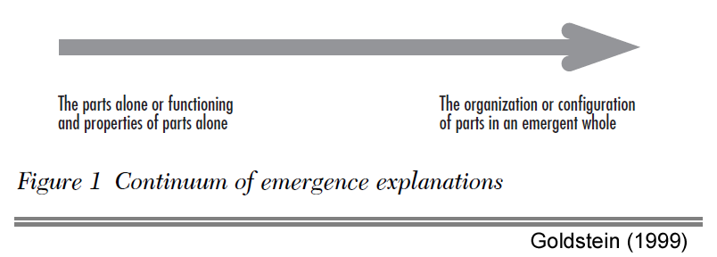
What is the value of the whole in terms of the values of the parts?

More specifically, given a finite set whose elements have assigned “values” v 1,…,v nv_1, \ldots, v_n and assigned “sizes” p 1,…,p np_1, \ldots, p_n (normalized to sum to 11), how can we assign a value σ(p,v)\sigma(\mathbf{p}, \mathbf{v}) to the set in a coherent way?

This seems like a very general question. But in fact, just a few sensible requirements on the function σ\sigma are enough to pin it down almost uniquely. And the answer turns out to be closely connected to existing mathematical concepts that you probably already know.

Let’s write

Δ n={(p 1,…,p n)∈ℝ n:p i≥0,∑p i=1} \Delta_n = \Bigl\{ (p_1, \ldots, p_n) \in \mathbb{R}^n : p_i \geq 0, \sum p_i = 1 \Bigr\}

for the set of probability distributions on {1,…,n}\{1, \ldots, n\}. Assuming that our “values” are positive real numbers, we’re interested in sequences of functions

(σ:Δ n×(0,∞) n→(0,∞)) n≥1 \Bigl( \sigma \colon \Delta_n \times (0, \infty)^n \to (0, \infty) \Bigr)_{n \geq 1}

that aggregate the values of the elements to give a value to the whole set. So, if the elements of the set have relative sizes p=(p 1,…,p n)\mathbf{p} = (p_1, \ldots, p_n) and values v=(v 1,…,v n)\mathbf{v} = (v_1, \ldots, v_n), then the value assigned to the whole set is σ(p,v)\sigma(\mathbf{p}, \mathbf{v}).

Here are some properties that it would be reasonable for σ\sigma to satisfy.

Homogeneity  The idea is that whatever “value” means, the value of the set and the value of the elements should be measured in the same units. For instance, if the elements are valued in kilograms then the set should be valued in kilograms too. A switch from kilograms to grams would then multiply both values by 1000. So, in general, we ask that

σ(p,cv)=cσ(p,v) \sigma(\mathbf{p}, c\mathbf{v}) = c \sigma(\mathbf{p}, \mathbf{v})

for all p∈Δ n\mathbf{p} \in \Delta_n, v∈(0,∞) n\mathbf{v} \in (0, \infty)^n and c∈(0,∞)c \in (0, \infty).

Monotonicity  The values of the elements are supposed to make a positive contribution to the value of the whole, so we ask that if v i≤v′ iv_i \leq v'_i for all ii then

σ(p,v)≤σ(p,v′) \sigma(\mathbf{p}, \mathbf{v}) \leq \sigma(\mathbf{p}, \mathbf{v}')

for all p∈Δ n\mathbf{p} \in \Delta_n.

Replication  Suppose that our nn elements have the same size and the same value, vv. Then the value of the whole set should be nvn v. This property says, among other things, that σ\sigma isn’t an average: putting in more elements of value vv increases the value of the whole set!

If σ\sigma is homogeneous, we might as well assume that v=1v = 1, in which case the requirement is that

σ((1/n,…,1/n),(1,…,1))=n. \sigma\bigl( (1/n, \ldots, 1/n), (1, \ldots, 1) \bigr) = n.

Modularity  This one’s a basic logical axiom, best illustrated by an example.

Imagine that we’re very ambitious and wish to evaluate the entire planet — or at least, the part that’s land. And suppose we already know the values and relative sizes of every country.

We could, of course, simply put this data into σ\sigma and get an answer immediately. But we could instead begin by evaluating each continent, and then compute the value of the planet using the values and sizes of the continents. If σ\sigma is sensible, this should give the same answer.

The notation needed to express this formally is a bit heavy. Let w∈Δ n\mathbf{w} \in \Delta_n; in our example, n=7n = 7 (or however many continents there are) and w=(w 1,…,w 7)\mathbf{w} = (w_1, \ldots, w_7) encodes their relative sizes. For each i=1,…,ni = 1, \ldots, n, let p i∈Δ k i\mathbf{p}^i \in \Delta_{k_i}; in our example, p i\mathbf{p}^i encodes the relative sizes of the countries on the iith continent. Then we get a probability distribution

w∘(p 1,…,p n)=(w 1p 1 1,…,w 1p k 1 1,…,w np 1 n,…,w np k n n)∈Δ k 1+⋯+k n, \mathbf{w} \circ (\mathbf{p}^1, \ldots, \mathbf{p}^n) = (w_1 p^1_1, \ldots, w_1 p^1_{k_1}, \,\,\ldots, \,\, w_n p^n_1, \ldots, w_n p^n_{k_n}) \in \Delta_{k_1 + \cdots + k_n},

which in our example encodes the relative sizes of all the countries on the planet. (Incidentally, this composition makes (Δ n)(\Delta_n) into an operad, a fact that we’ve discussed many times before on this blog.) Also let

v 1=(v 1 1,…,v k 1 1)∈(0,∞) k 1,…,v n=(v 1 n,…,v k n n)∈(0,∞) k n. \mathbf{v}^1 = (v^1_1, \ldots, v^1_{k_1}) \in (0, \infty)^{k_1}, \,\,\ldots,\,\, \mathbf{v}^n = (v^n_1, \ldots, v^n_{k_n}) \in (0, \infty)^{k_n}.

In the example, v j iv^i_j is the value of the jjth country on the iith continent. Then the value of the iith continent is σ(p i,v i)\sigma(\mathbf{p}^i, \mathbf{v}^i), so the axiom is that

σ(w∘(p 1,…,p n),(v 1 1,…,v k 1 1,…,v 1 n,…,v k n n))=σ(w,(σ(p 1,v 1),…,σ(p n,v n))). \sigma \bigl( \mathbf{w} \circ (\mathbf{p}^1, \ldots, \mathbf{p}^n), (v^1_1, \ldots, v^1_{k_1}, \ldots, v^n_1, \ldots, v^n_{k_n}) \bigr) = \sigma \Bigl( \mathbf{w}, \bigl( \sigma(\mathbf{p}^1, \mathbf{v}^1), \ldots, \sigma(\mathbf{p}^n, \mathbf{v}^n) \bigr) \Bigr).

The left-hand side is the value of the planet calculated in a single step, and the right-hand side is its value when calculated in two steps, with continents as the intermediate stage.

Symmetry  It shouldn’t matter what order we list the elements in. So it’s natural to ask that

σ(p,v)=σ(pτ,vτ) \sigma(\mathbf{p}, \mathbf{v}) = \sigma(\mathbf{p} \tau, \mathbf{v} \tau)

for any τ\tau in the symmetric group S nS_n, where the right-hand side refers to the obvious S nS_n-actions.

Absent elements should count for nothing! In other words, if p 1=0p_1 = 0 then we should have

σ((p 1,…,p n),(v 1,…,v n))=σ((p 2,…,p n),(v 2,…,v n)). \sigma\bigl( (p_1, \ldots, p_n), (v_1, \ldots, v_n)\bigr) = \sigma\bigl( (p_2, \ldots, p_n), (v_2, \ldots, v_n)\bigr).

This isn’t quite triival. I haven’t yet given you any examples of the kind of function that σ\sigma might be, but perhaps you already have in mind a simple one like this:

σ(p,v)=v 1+⋯+v n. \sigma(\mathbf{p}, \mathbf{v}) = v_1 + \cdots + v_n.

In words, the value of the whole is simply the sum of the values of the parts, regardless of their sizes. But if σ\sigma is to have the “absent elements” property, this won’t do. (Intuitively, if p i=0p_i = 0 then we shouldn’t count v iv_i in the sum, because the iith element isn’t actually there.) So we’d better modify this example slightly, instead taking

σ(p,v)=∑ i:p i>0v i. \sigma(\mathbf{p}, \mathbf{v}) = \sum_{i \,:\, p_i \gt 0} v_i.

This function (or rather, sequence of functions) does have the “absent elements” property.

Continuity in positive probabilities  Finally, we ask that for each v∈(0,∞) n\mathbf{v} \in (0, \infty)^n, the function σ(−,v)\sigma(-, \mathbf{v}) is continuous on the interior of the simplex Δ n\Delta_n, that is, continuous over those probability distributions p\mathbf{p} such that p 1,…,p n>0p_1, \ldots, p_n \gt 0.

Why only over the interior of the simplex? Basically because of natural examples of σ\sigma like the one just given, which is continuous on the interior of the simplex but not the boundary. Generally, it’s sometimes useful to make a sharp, discontinuous distinction between the cases p i>0p_i \gt 0 (presence) and p i=0p_i = 0 (absence).

 

Arrow’s famous theorem states that a few apparently mild conditions on a voting system are, in fact, mutually contradictory. The mild conditions above are not mutually contradictory. In fact, there’s a one-parameter family σ q\sigma_q of functions each of which satisfies these conditions. For real q≠1q \neq 1, the definition is

σ q(p,v)=(∑ i:p i>0p i qv i 1−q) 1/(1−q). \sigma_q(\mathbf{p}, \mathbf{v}) = \Bigl( \sum_{i \,:\, p_i \gt 0} p_i^q v_i^{1 - q} \Bigr)^{1/(1 - q)}.

For instance, σ 0\sigma_0 is the example of σ\sigma given above.

The formula for σ q\sigma_q is obviously invalid at q=1q = 1, but it converges to a limit as q→1q \to 1, and we define σ 1(p,v)\sigma_1(\mathbf{p}, \mathbf{v}) to be that limit. Explicitly, this gives

σ 1(p,v)=∏ i:p i>0(v i/p i) p i. \sigma_1(\mathbf{p}, \mathbf{v}) = \prod_{i \,:\, p_i \gt 0} (v_i/p_i)^{p_i}.

In the same way, we can define σ −∞\sigma_{-\infty} and σ ∞\sigma_\infty as the appropriate limits:

σ −∞(p,v)=max i:p i>0v i/p i,σ ∞(p,v)=min i:p i>0v i/p i. \sigma_{-\infty}(\mathbf{p}, \mathbf{v}) = \max_{i \,:\, p_i \gt 0} v_i/p_i, \qquad \sigma_{\infty}(\mathbf{p}, \mathbf{v}) = \min_{i \,:\, p_i \gt 0} v_i/p_i.

And it’s easy to check that for each q∈[−∞,∞]q \in [-\infty, \infty], the function σ q\sigma_q satisfies all the natural conditions listed above.

These functions σ q\sigma_q might be unfamiliar to you, but they have some special cases that are quite well-explored. In particular:

• Suppose you’re in a situation where the elements don’t have “sizes”. Then it would be natural to take p\mathbf{p} to be the uniform distribution u n=(1/n,…,1/n)\mathbf{u}_n = (1/n, \ldots, 1/n). In that case, σ q(u n,v)=const⋅(∑v i 1−q) 1/(1−q), \sigma_q(\mathbf{u}_n, \mathbf{v}) = const \cdot \bigl( \sum v_i^{1 - q} \bigr)^{1/(1 - q)}, where the constant is a certain power of nn. When q≤0q \leq 0, this is exactly a constant times ‖v‖ 1−q\|\mathbf{v}\|_{1 - q}, the (1−q)(1 - q)-norm of the vector v\mathbf{v}.

• Suppose you’re in a situation where the elements don’t have “values”. Then it would be natural to take v\mathbf{v} to be 1=(1,…,1)\mathbf{1} = (1, \ldots, 1). In that case, σ q(p,1)=(∑p i q) 1/(1−q). \sigma_q(\mathbf{p}, \mathbf{1}) = \bigl( \sum p_i^q \bigr)^{1/(1 - q)}. This is the quantity that ecologists know as the Hill number of order qq and use as a measure of biological diversity. Information theorists know it as the exponential of the Rényi entropy of order qq, the special case q=1q = 1 being Shannon entropy. And actually, the general formula for σ q\sigma_q is very closely related to Rényi relative entropy (which Wikipedia calls Rényi divergence).

Anyway, the big — and as far as I know, new — result is:

Theorem  The functions σ q\sigma_q are the only functions σ\sigma with the seven properties above.

So although the properties above don’t seem that demanding, they actually force our notion of “aggregate value” to be given by one of the functions in the family (σ q) q∈[−∞,∞](\sigma_q)_{q \in [-\infty, \infty]}. And although I didn’t even mention the notions of diversity or entropy in my justification of the axioms, they come out anyway as special cases.

I covered all this yesterday in the tenth and penultimate installment of the functional equations course that I’m giving. It’s written up on pages 38–42 of the notes so far. There you can also read how this relates to more realistic measures of biodiversity than the Hill numbers. Plus, you can see an outline of the (quite substantial) proof of the theorem above.

The ability to learn tasks in a sequential fashion is crucial to the development of artificial intelligence. Until now neural networks have not been capable of this and it has been widely thought that catastrophic forgetting is an inevitable feature of connectionist models. We show that it is possible to...

A sperm-driven micromotor is presented as cargo-delivery system for the treatment of gynecological cancers. This particular hybrid micromotor is appealing to treat diseases in the female reproductive tract, the physiological environment that sperm cells are naturally adapted to swim in. Here, the single sperm cell serves as an active drug carrier and as driving force, taking advantage of its swimming capability, while a laser-printed microstructure coated with a nanometric layer of iron is used to guide and release the sperm in the desired area by an external magnet and structurally imposed mechanical actuation, respectively. The printed tubular microstructure features four arms which release the drug-loaded sperm cell in situ when they bend upon pushing against a tumor spheroid, resulting in the drug delivery, which occurs when the sperm squeezes through the cancer cells and fuses with cell membrane. Sperms also offer higher drug encapsulation capability and carrying stability compared to other nano and microcarriers, minimizing toxic effects and unwanted drug accumulation. Moreover, sperms neither express pathogenic proteins nor proliferate to form undesirable colonies, unlike other cells or microorganisms do, making this bio-hybrid system a unique and biocompatible cargo delivery platform for various biomedical applications, especially in gynecological healthcare.

Persistent homology (PH) is a method used in topological data analysis (TDA) to study qualitative features of data that persist across multiple scales. It is robust to perturbations of input data, independent of dimensions and coordinates, and provides a compact representation of the qualitative features of the input. The computation of PH is an open area with numerous important and fascinating challenges. The field of PH computation is evolving rapidly, and new algorithms and software implementations are being updated and released at a rapid pace. The purposes of our article are to (1) introduce theory and computational methods for PH to a broad range of computational scientists and (2) provide benchmarks of state-of-the-art implementations for the computation of PH. We give a friendly introduction to PH, navigate the pipeline for the computation of PH with an eye towards applications, and use a range of synthetic and real-world data sets to evaluate currently available open-source implementations for the computation of PH. Based on our benchmarking, we indicate which algorithms and implementations are best suited to different types of data sets. In an accompanying tutorial, we provide guidelines for the computation of PH. We make publicly available all scripts that we wrote for the tutorial, and we make available the processed version of the data sets used in the benchmarking.

“You” is one of the most common words in the English language. Although it typically refers to the person addressed (“How are you?”), “you” is also used to make timeless statements about people in general (“You win some, you lose some.”). Here, we demonstrate that this ubiquitous but understudied linguistic device, known as “generic-you,” has important implications for how people derive meaning from experience. Across six experiments, we found that generic-you is used to express norms in both ordinary and emotional contexts and that producing generic-you when reflecting on negative experiences allows people to “normalize” their experience by extending it beyond the self. In this way, a simple linguistic device serves a powerful meaning-making function. Authors: Ariana Orvell, Ethan Kross, Susan A. Gelman

Is there a link between the color of a taxi and how many accidents it has? An analysis of 36 mo of detailed taxi, driver, and accident data (comprising millions of data points) from the largest taxi company in Singapore suggests that there is an explicit link. Yellow taxis had...

Florida edition.

As punishment, four corrections officers — John Fan Fan, Cornelius Thompson, Ronald Clarke and Edwina Williams — kept Rainey in that shower for two full hours. Rainey was heard screaming "Please take me out! I can’t take it anymore!” and kicking the shower door. Inmates said prison guards laughed at Rainey and shouted "Is it hot enough?"

Rainey died inside that shower. He was found crumpled on the floor. When his body was pulled out, nurses said there were burns on 90 percent of his body. A nurse said his body temperature was too high to register with a thermometer. And his skin fell off at the touch.

But in an unconscionable decision, Miami-Dade State Attorney Katherine Fernandez Rundle's office announced Friday that the four guards who oversaw what amounted to a medieval-era boiling will not be charged with a crime.

Observation of discrete time-crystalline order in a disordered dipolar many-body system

Nature 543, 7644 (2017). doi:10.1038/nature21426

Authors: Soonwon Choi, Joonhee Choi, Renate Landig, Georg Kucsko, Hengyun Zhou, Junichi Isoya, Fedor Jelezko, Shinobu Onoda, Hitoshi Sumiya, Vedika Khemani, Curt von Keyserlingk, Norman Y. Yao, Eugene Demler & Mikhail D. Lukin

Understanding quantum dynamics away from equilibrium is an outstanding challenge in the modern physical sciences. Out-of-equilibrium systems can display a rich variety of phenomena, including self-organized synchronization and dynamical phase transitions. More recently, advances in the controlled manipulation of isolated many-body systems have enabled detailed studies of non-equilibrium phases in strongly interacting quantum matter; for example, the interplay between periodic driving, disorder and strong interactions has been predicted to result in exotic ‘time-crystalline’ phases, in which a system exhibits temporal correlations at integer multiples of the fundamental driving period, breaking the discrete time-translational symmetry of the underlying drive. Here we report the experimental observation of such discrete time-crystalline order in a driven, disordered ensemble of about one million dipolar spin impurities in diamond at room temperature. We observe long-lived temporal correlations, experimentally identify the phase boundary and find that the temporal order is protected by strong interactions. This order is remarkably stable to perturbations, even in the presence of slow thermalization. Our work opens the door to exploring dynamical phases of matter and controlling interacting, disordered many-body systems.

Identifying causal relationships from observational time series data is a key problem in disciplines such as climate science or neuroscience, where experiments are often not possible. Data-driven causal inference is challenging since datasets are often high-dimensional and nonlinear with limited sample sizes. Here we introduce a novel method that flexibly combines linear or nonlinear conditional independence tests with a causal discovery algorithm that allows to reconstruct causal networks from large-scale time series datasets. We validate the method on a well-established climatic teleconnection connecting the tropical Pacific with extra-tropical temperatures and using large-scale synthetic datasets mimicking the typical properties of real data. The experiments demonstrate that our method outperforms alternative techniques in detection power from small to large-scale datasets and opens up entirely new possibilities to discover causal networks from time series across a range of research fields.

Computing: A faster brain-inspired computer

Nature 542, 7642 (2017). doi:10.1038/542394b

A computer that mimics the way the brain works, and contains both optical and electronic parts, can recognize simple speech three times faster than earlier devices that used only optical components.Reservoir computers use neural networks made of interconnected units that relay signals in recurrent,

The post *Fascism: 100 questions asked and answered* appeared first on Marginal REVOLUTION.

The post *Eurasian Mission*, by Alexander Dugin appeared first on Marginal REVOLUTION.

Each of our movements is selected from any number of alternative movements. Some studies have shown evidence that the central nervous system (CNS) chooses to make the specific movements that are least affected by motor noise. Previous results showing that the CNS has a natural tendency to minimize the effects of noise make the direct prediction that if the relationship between movements and noise were to change, the specific movements people learn to make would also change in a predictable manner. Indeed, this has been shown for well-practiced movements such as reaching. Here, we artificially manipulated the relationship between movements and visuomotor noise by adding noise to a motor task in a novel redundant geometry such that there arose a single control policy that minimized the noise. This allowed us to see whether, for a novel motor task, people could learn the specific control policy that minimized noise or would need to employ other compensation strategies to overcome the added noise. As predicted, subjects were able to learn movements that were biased toward the specific ones that minimized the noise, suggesting not only that the CNS can learn to minimize the effects of noise in a novel motor task but also that artificial visuomotor noise can be a useful tool for teaching people to make specific movements. Using noise as a teaching signal promises to be useful for rehabilitative therapies and movement training with human-machine interfaces.

NEW & NOTEWORTHY Many theories argue that we choose to make the specific movements that minimize motor noise. Here, by changing the relationship between movements and noise, we show that people actively learn to make movements that minimize noise. This not only provides direct evidence for the theories of noise minimization but presents a way to use noise to teach specific movements to improve rehabilitative therapies and human-machine interface control.

This week I’m giving a talk on biology and information:

• John Baez, Biology as information dynamics, talk for Biological Complexity: Can it be Quantified?, a workshop at the Beyond Center, 2 February 2017.

While preparing this talk, I discovered a cool fact. I doubt it’s new, but I haven’t exactly seen it elsewhere. I came up with it while trying to give a precise and general statement of ‘Fisher’s fundamental theorem of natural selection’. I won’t start by explaining that theorem, since my version looks rather different than Fisher’s, and I came up with mine precisely because I had trouble understanding his. I’ll say a bit more about this at the end.

Here’s my version:

The square of the rate at which a population learns information is the variance of its fitness.

This is a nice advertisement for the virtues of diversity: more variance means faster learning. But it requires some explanation!

The setup

Let’s start by assuming we have different kinds of self-replicating entities with populations As usual, these could be all sorts of things:

• molecules of different chemicals
• organisms belonging to different species
• genes of different alleles
• restaurants belonging to different chains
• people with different beliefs
• game-players with different strategies
• etc.

I’ll call them replicators of different species.

Let’s suppose each population is a function of time that grows at a rate equal to this population times its ‘fitness’. I explained the resulting equation back in Part 9, but it’s pretty simple:

Here is a completely arbitrary smooth function of all the populations! We call it the fitness of the ith species.

This equation is important, so we want a short way to write it. I’ll often write simply as and simply as With these abbreviations, which any red-blooded physicist would take for granted, our equation becomes simply this:

Next, let be the probability that a randomly chosen organism is of the ith species:

Starting from our equation describing how the populations evolve, we can figure out how these probabilities evolve. The answer is called the replicator equation:

Here is the average fitness of all the replicators, or mean fitness:

In what follows I’ll abbreviate the replicator equation as follows:

The result

Okay, now let’s figure out how fast the probability distribution

changes with time. For this we need to choose a way to measure the length of the vector

And here information geometry comes to the rescue! We can use the Fisher information metric, which is a Riemannian metric on the space of probability distributions.

I’ve talked about the Fisher information metric in many ways in this series. The most important fact is that as a probability distribution changes with time, its speed

as measured using the Fisher information metric can be seen as the rate at which information is learned. I’ll explain that later. Right now I just want a simple formula for the Fisher information metric. Suppose and are two tangent vectors to the point in the space of probability distributions. Then the Fisher information metric is given as follows:

Using this we can calculate the speed at which moves when it obeys the replicator equation. Actually the square of the speed is simpler:

The answer has a nice meaning, too! It’s just the variance of the fitness: that is, the square of its standard deviation.

So, if you’re willing to buy my claim that the speed is the rate at which our population learns new information, then we’ve seen that the square of the rate at which a population learns information is the variance of its fitness!

Fisher’s fundamental theorem

Now, how is this related to Fisher’s fundamental theorem of natural selection? First of all, what is Fisher’s fundamental theorem? Here’s what Wikipedia says about it:

It uses some mathematical notation but is not a theorem in the mathematical sense.

It states:

“The rate of increase in fitness of any organism at any time is equal to its genetic variance in fitness at that time.”

Or in more modern terminology:

“The rate of increase in the mean fitness of any organism at any time ascribable to natural selection acting through changes in gene frequencies is exactly equal to its genetic variance in fitness at that time”.

Largely as a result of Fisher’s feud with the American geneticist Sewall Wright about adaptive landscapes, the theorem was widely misunderstood to mean that the average fitness of a population would always increase, even though models showed this not to be the case. In 1972, George R. Price showed that Fisher’s theorem was indeed correct (and that Fisher’s proof was also correct, given a typo or two), but did not find it to be of great significance. The sophistication that Price pointed out, and that had made understanding difficult, is that the theorem gives a formula for part of the change in gene frequency, and not for all of it. This is a part that can be said to be due to natural selection

Price’s paper is here:

• George R. Price, Fisher’s ‘fundamental theorem’ made clear, Annals of Human Genetics 36 (1972), 129–140.

I don’t find it very clear, perhaps because I didn’t spend enough time on it. But I think I get the idea.

My result is a theorem in the mathematical sense, though quite an easy one. I assume a population distribution evolves according to the replicator equation and derive an equation whose right-hand side matches that of Fisher’s original equation: the variance of the fitness.

But my left-hand side is different: it’s the square of the speed of the corresponding probability distribution, where speed is measured using the ‘Fisher information metric’. This metric was discovered by the same guy, Ronald Fisher, but I don’t think he used it in his work on the fundamental theorem!

Something a bit similar to my statement appears as Theorem 2 of this paper:

• Marc Harper, Information geometry and evolutionary game theory.

and for that theorem he cites:

• Josef Hofbauer and Karl Sigmund, Evolutionary Games and Population Dynamics, Cambridge University Press, Cambridge, 1998.

However, his Theorem 2 really concerns the rate of increase of fitness, like Fisher’s fundamental theorem. Moreover, he assumes that the probability distribution flows along the gradient of a function, and I’m not assuming that. Indeed, my version applies to situations where the probability distribution moves round and round in periodic orbits!

Relative information and the Fisher information metric

The key to generalizing Fisher’s fundamental theorem is thus to focus on the speed at which moves, rather than the increase in fitness. Why do I call this speed the ‘rate at which the population learns information’? It’s because we’re measuring this speed using the Fisher information metric, which is closely connected to relative information, also known as relative entropy or the Kullback–Leibler divergence.

I explained this back in Part 7, but that explanation seems hopelessly technical to me now, so here’s a faster one, which I created while preparing my talk.

The information of a probability distribution relative to a probability distribution is

It says how much information you learn if you start with a hypothesis saying that the probability of the ith situation was and then update this to a new hypothesis

Now suppose you have a hypothesis that’s changing with time in a smooth way, given by a time-dependent probability Then a calculation shows that

for all times . This seems paradoxical at first. I like to jokingly put it this way:

To first order, you’re never learning anything.

However, as long as the velocity is nonzero, we have

so we can say

To second order, you’re always learning something… unless your opinions are fixed.

This lets us define a ‘rate of learning’—that is, a ‘speed’ at which the probability distribution moves. And this is precisely the speed given by the Fisher information metric!

In other words:

where the length is given by Fisher information metric. Indeed, this formula can be used to define the Fisher information metric. From this definition we can easily work out the concrete formula I gave earlier.

In summary: as a probability distribution moves around, the relative information between the new probability distribution and the original one grows approximately as the square of time, not linearly. So, to talk about a ‘rate at which information is learned’, we need to use the above formula, involving a second time derivative. This rate is just the speed at which the probability distribution moves, measured using the Fisher information metric. And when we have a probability distribution describing how many replicators are of different species, and it’s evolving according to the replicator equation, this speed is also just the variance of the fitness!

Dermatologist-level classification of skin cancer with deep neural networks

Nature 542, 7639 (2017). doi:10.1038/nature21056

Authors: Andre Esteva, Brett Kuprel, Roberto A. Novoa, Justin Ko, Susan M. Swetter, Helen M. Blau & Sebastian Thrun

Skin cancer, the most common human malignancy, is primarily diagnosed visually, beginning with an initial clinical screening and followed potentially by dermoscopic analysis, a biopsy and histopathological examination. Automated classification of skin lesions using images is a challenging task owing to the fine-grained variability in the appearance of skin lesions. Deep convolutional neural networks (CNNs) show potential for general and highly variable tasks across many fine-grained object categories. Here we demonstrate classification of skin lesions using a single CNN, trained end-to-end from images directly, using only pixels and disease labels as inputs. We train a CNN using a dataset of 129,450 clinical images—two orders of magnitude larger than previous datasets—consisting of 2,032 different diseases. We test its performance against 21 board-certified dermatologists on biopsy-proven clinical images with two critical binary classification use cases: keratinocyte carcinomas versus benign seborrheic keratoses; and malignant melanomas versus benign nevi. The first case represents the identification of the most common cancers, the second represents the identification of the deadliest skin cancer. The CNN achieves performance on par with all tested experts across both tasks, demonstrating an artificial intelligence capable of classifying skin cancer with a level of competence comparable to dermatologists. Outfitted with deep neural networks, mobile devices can potentially extend the reach of dermatologists outside of the clinic. It is projected that 6.3 billion smartphone subscriptions will exist by the year 2021 (ref. 13) and can therefore potentially provide low-cost universal access to vital diagnostic care.

Evocative.  Res ipsa loquitur.

Photo credit Mohammed Al-Khatieb/AFP/Getty Images, via The Huffington Post.

Recent progress in applying machine learning for jet physics has been built upon an analogy between calorimeters and images. In this work, we present a novel class of recursive neural networks built instead upon an analogy between QCD and natural languages. In the analogy, four-momenta are like words and the clustering history of sequential recombination jet algorithms is like the parsing of a sentence. Our approach works directly with the four-momenta of a variable-length set of particles, and the jet-based tree structure varies on an event-by-event basis. Our experiments highlight the flexibility of our method for building task-specific jet embeddings and show that recursive architectures are significantly more accurate and data efficient than previous image-based networks. We extend the analogy from individual jets (sentences) to full events (paragraphs), and show for the first time an event-level classifier operating on all the stable particles produced in an LHC event.

This is my talk for the workshop Biological Complexity: Can It Be Quantified?

• John Baez, Biology as information dynamics, 2 February 2017.

Abstract. If biology is the study of self-replicating entities, and we want to understand the role of information, it makes sense to see how information theory is connected to the ‘replicator equation’—a simple model of population dynamics for self-replicating entities. The relevant concept of information turns out to be the information of one probability distribution relative to another, also known as the Kullback–Leibler divergence. Using this we can get a new outlook on free energy, see evolution as a learning process, and give a clean general formulation of Fisher’s fundamental theorem of natural selection.

For more, read:

• Marc Harper, The replicator equation as an inference dynamic.

• Marc Harper, Information geometry and evolutionary game theory.

• Barry Sinervo and Curt M. Lively, The rock-paper-scissors game and the evolution of alternative male strategies, Nature 380 (1996), 240–243.

• John Baez, Diversity, entropy and thermodynamics.

• John Baez, Information geometry.

The last reference contains proofs of the equations shown in red in my slides.
In particular, Part 16 contains a proof of my updated version of Fisher’s fundamental theorem.

Nature Neuroscience 20, 287 (2017). doi:10.1038/nn.4458

Authors: Elseline Hoekzema, Erika Barba-Müller, Cristina Pozzobon, Marisol Picado, Florencio Lucco, David García-García, Juan Carlos Soliva, Adolf Tobeña, Manuel Desco, Eveline A Crone, Agustín Ballesteros, Susanna Carmona & Oscar Vilarroya

I’m currently reading a preprint by a deservedly very well-respected and highly-reputed mathematician. It’s enjoyable, inspirational, and wonderful. The ideas that it expresses have been haunting and taunting me for years.

For various reasons, I have the impression that it was not wholly written while the author was wholly sober. That’s OK; I’ll judge the paper for what it is, not on how it was written. But it leads me to wonder: how common is this? In literature, it’s a well-established tradition to the point of cliché. For instance, here’s Ernest Hemingway —

— giving a cocktail recipe for difficult political times (1937), “to be enjoyed from 11:00am on”. You can find countless examples of fiction writers enthusing about chemically-assisted escape from the so-called real world.

But mathematics prides itself on sharpness and precision in counterpoint to creativity. We love to say that we’re more creative than poets, but a piece of mathematics is in deep trouble if it’s logically wrong. So where does drugged, drunk or hallucinatory mathematics fit into our mathematicians’ culture?

Biochemical oscillations are prevalent in living organisms. Systems with a small number of constituents cannot sustain coherent oscillations for an indefinite time because of fluctuations in the period of oscillation. We show that the number of coherent oscillations that quantifies the precision of the oscillator is universally bounded by the thermodynamic force that drives the system out of equilibrium and by the topology of the underlying biochemical network of states. Our results are valid for arbitrary Markov processes, which are commonly used to model biochemical reactions. We apply our results to a model for a single KaiC protein and to an activator-inhibitor model that consists of several molecules. From a mathematical perspective, based on strong numerical evidence, we conjecture a universal constraint relating the imaginary and real parts of the first non-trivial eigenvalue of a stochastic matrix.

Author(s): Thomas McGrath, Nick S. Jones, Pieter Rein ten Wolde, and Thomas E. Ouldridge

An enzyme in a chemical bath can act as an autonomous biochemical device that exploits information to do work.

[Phys. Rev. Lett. 118, 028101] Published Tue Jan 10, 2017

Neural Computation, Volume 29, Issue 3, Page 861-866, March 2017.

guest post by Nadja Kutz

This blog post is based on a thread in the Azimuth Forum.

The current theories about the Sun’s life-time indicate that the Sun will turn into a red giant in about 5 billion years. How and when this process is going to be destructive to the Earth is still debated. Apparently, according to more or less current theories, there has been a quasilinear increase in luminosity. On page 3 of

• K.-P. Schröder and Robert Connon Smith, Distant future of the Sun and Earth revisited, 2008.

we read:

The present Sun is increasing its average luminosity at a rate of 1% in every 110 million years, or 10% over the next billion years.

Unfortunately I feel a bit doubtful about this, in particular after I looked at some irradiation measurements. But let’s recap a bit.

In the Azimuth Forum I asked for information about solar irradiance measurements . Why I was originally interested in how bright the Sun is shining is a longer story, which includes discussions about the global warming potential of methane. For this post I prefer to omit this lengthy historical survey about my original motivations (maybe I’ll come back to this later). Meanwhile there is an also a newer reason why I am interested in solar irradiance measurements, which I want to talk about here.

Strictly speaking I was not only interested in knowing more about how bright the sun is shining, but how bright each of its ‘components’ is shining. That is, I wanted to see spectrally resolved solar irradiance measurements—and in particular, measurements in the range between the wavelengths of roughly 650 and 950 nanometers.

This led me to the the Sorce mission, which is a NASA sponsored satellite mission, whose website is located at the University of Colorado. The website very nicely provides an interactive interface including a fairly clear and intuitive LISIRD interactive app with which the spectral measurements of the Sun can be studied.

As a side remark I should mention that this NASA mission belongs to the NASA Earth Science mission, which is currently threatened to be scrapped.

By using this app, I found in the 650–950 nanometer range a very strange rise in radiation between 2003 and 2016, which happened mainly in the last 2-3 years. You can see this rise here (click to enlarge):

Now, fluctuations within certain spectral ranges within the Sun’s spectrum are not news. Here, however, it looked as if a rather stable range suddenly started to change rather “dramatically”.

I put the word “dramatically” in quotes for a couple of reasons.

Spectral measurements are complicated and prone to measurement errors. Subtle issues of dirty lenses and the like are already enough to suggest that this is no easy feat, so that this strange rise might easily be due to a measurement failure. Moreover, as I said, it looked as this was a fairly stable range over the course of ten years. But maybe this new rise in irradiation is part of the 11 years solar cycle, i.e., a common phenomenon. In addition, although the rise looks big, it may overall still be rather subtle.

So: how subtle or non-subtle is it then?

In order to assess that, I made a quick estimate (see the Forum discussion) and found that if all the additional radiation would reach the ground (which of course it doesn’t due to absorption), then on 1000 square meters you could easily power a lawn mower with that subtle change! I.e., my estimate was 1200 watts for that patch of lawn. Whoa!

That was disconcerting enough to download the data and linearly interpolate it and calculate the power of that change. I wrote a program in Javascript to do that. The computer calculations revealed an answer of 1000 watts, i.e., my estimate was fairly close. Whoa again!

How does this translate to overall changes in solar irradiance? Some increase had already been noticed. NASA wrote 2003 on its webpage:

Although the inferred increase of solar irradiance in 24 years, about 0.1 percent, is not enough to cause notable climate change, the trend would be important if maintained for a century or more.

That was 13 years ago.

I now used my program to calculate the irradiance for one day in 2016 between the wavelengths of 180.5 nm and 1797.62 nm, a quite big part of the solar spectrum, and got the value 627 W/m². I computed the difference between this and one day in 2003, approximately one solar cycle earlier. I got 0.61 W/m², which is 0.1% in 13 years, rather then 24 years. Of course this is not an average value, and not really well adjusted to the sun cycle, and fluctuations play a big role in some parts of the spectrum, but well—this might indicate that the overall rate of rise in solar radiation may have doubled. Likewise concerning the question of the sun’s luminosity: for assessing luminosity one would need to take the concrete satellite-earth orbit at the day of measurement into account, as the distance to the sun varies. But still, on a first glance this all appears disconcerting.

Given that this spectral range has for example an overlap with the absorption of water (clouds!), this should at least be discussed.

See how the spectrum splits into a purple and dark red line in the lower circle? (Click to enlarge.)

The upper circle displays another rise, which is discussed in the forum.

So concluding, all this looks as if this needs to be monitored a bit more closely. It is important to see whether these rises in irradiance are also displayed in other measurements, so I asked in the Azimuth Forum, but so far have gotten no answer.

The Russian Wikipedia site about solar irradiance unfortunately contains no links to Russian satellite missions (if I haven’t overlooked something), and there exists no Chinese or Indian Wikipedia about solar irradiance. I also couldn’t find any publicly accessible spectral irradiance measurements on the ESA website (although they have some satellites out there). In December I wrote an email to the head of the section solar radiometry of the World Radiation Center (WRC) Wolfgang Finsterle, but I’ve had no answer yet.

In short: if you know about publicly available solar spectral irradiance measurements other than the LISIRD ones, then please let me know.