20 Jun 07:00

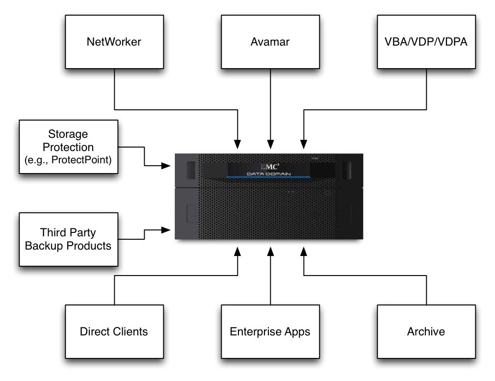
One target to rule them all

by Preston de Guise

Introduction

It’s true there are some data types that broadly aren’t suitable to sending to Data Domain – any more than they’re suitable for sending to any other deduplication appliance or system within any environment. Large imaging data and video files will yield minimal deduplication except over successive backups (assuming static data), and compressed and/or encrypted data aren’t all suited either.

But the majority of data within most organisations is suited for writing to Data Domain systems.

Years ago when EMC purchased Data Domain, I don’t think anyone anticipated just what they had in mind for the appliance. I certainly didn’t – and I’d been involved in the backup industry for probably 15 years at that point. Deduplication had been kicking around for several years, but it hadn’t been mainstreamed to the degree EMC has achieved.

The numbers practically speak for themselves. Data Domain represents an overwhelming lions share of the deduplication appliance space – but I’m not going to quote numbers here. I’m going to talk about the architectural vision of Data Domain.

As a target-only appliance, Data Domain represents considerable advantage to any business that deploys it, but that’s just the tip of the iceberg. The real magic happens when we start to consider the simple fact that a Data Domain is not a dumb appliance. EMC have chosen to harness the platform to deliver maximum bang for buck for any company that walks down that path.

May the source be with you

Target based deduplication works brilliantly for drastically reducing the total amount of data stored, but it still results in that data being sent. Avamar demonstrates this overwhelmingly – its source based deduplication backup process is unbelievably efficient and powerful and is a powerfully attractive choice for many businesses, particularly those in the xaaS industry.

Data Domain’s Boost functionality extends its deduplication technology up to the origin of the data. For products like NetWorker, Avamar and VDP/VDPA, this goes right to the source. (For third party products such as NetBackup, it covers the media servers.)

If Boost had stopped at NetWorker and Avamar integration, it would have been a remarkably powerful efficiency hook for many businesses, but there’s more power to be had. The extension of Data Domain Boost to include support for enterprise applications such as Oracle, SQL Server, SAP, etc., provides unparalleled extensibility in the backup space to organisations. It also means that businesses who have deployed other backup technologies but leverage the power of Data Domain deduplication in their data protection strategy can get direct client deduplication performance for what is often their most mission critical systems and applications.

I’m the first to admit that I’ve spent years trying to convince DBAs to hand over control of their application backups to NetWorker administrators. It’s a discussion I’ve won as much as I’ve lost, but the Data Domain plugins for databases have proven one key lesson: when I’ve ‘lost’ that discussion it’s not been through lack of conviction, but through lack of process. DBAs are all for efficiencies in the backup process, but given the enterprise criticality of databases in so many organisations, much of the push back on backup centralisation has been from a lack of control of the process.

The Boost application plugins get past that by allowing a business to make the decision to integrate their application backups into centralised backup storage while allowing for highly granular control of the backup process through the agreed and trusted scheduling methods that offer considerably more granular and flexible controls. Backup products offer scheduling, of course, but they’re not meant to be the bees knees of scheduling that you’ll find in products devoted solely to that purpose. That’s what DBAs have mostly resisted. (This, for what it’s worth, is the difference between app-centric aspects to backup and recovery and a decentralised backup ‘system’.)

Here’s where we’re at with Data Domain – it now sits at a nexus in the Data Centre for data protection and nearline archival storage:

(Yes, it’s even very well suited for archival workloads.)

NetWorker, Avamar, VDP/VDPA, Client Direct, Enterprise Apps – I could go on – Data Domain sits at the centre ready to receive the data you want to send to it.

But that diagram isn’t quite complete. To truly get the maximised efficiency out of Data Domain, the picture really should look more like this:

That’s right – logically, a Data Domain solution will have at least two Data Domains in it, so that whatever you’re protecting via the Data Domain will itself be protected. Now, by itself, Data Domain offers excellent protection for the data you’re storing, but unlike what most people think of on this front, RAID-6 storage protection is just the tip of the iceberg. RAID-6 is nice – it protects you from two drive failures at any point. On top of that though, you have the Data Invulnerability Architecture that you’ll hear EMC folks talk about quite regularly – that’s the magic sauce. The Data Domain doesn’t just sit there storing your data: it stores it, it checks it, it reads it again, and it checks it as part of regular verification. (If you want to compare it to tape, imagine having a tape library big enough to store every tape you keep for retention and constantly sits there loading all the tapes and confirming all the data can be read back.)

But we all know in the data protection world that you still need that added protection of keeping a second copy of that data, regardless of whether that’s for compliance or for true disaster protection. In terms of absolute efficiency, the absolute best way you’ll get a secondary copy of that data is via the global deduplicated replication offered between two Data Domains. (For what it’s worth, that’s where some companies make the mistake of deploying tape as their secondary copy from an original backup target of Data Domain: what’s the point of deploying efficient deduplication if the first thing you’re going to do is rehydrate all the content again?)

Aside: Coming back to encryption and compression

Earlier I said that compressed and encrypted workloads aren’t necessarily suited to Data Domain. That’s true, but that usually reflects an opportunity to revisit the process and thinking behind those workloads.

Compression is typically used in a data streaming activity for data protection because of a requirement to minimise the amount of data going across the network. Boost eliminates that need by doing something better than compression at the client side – deduplication. Deduplication doesn’t just compress the original data, but it substantially reduces the original data by not even bothering to send data that already exists at the target. For instance, if I turn my attention to Oracle, the two most common reasons why DBAs will create compressed Oracle backups are:

(a) They’re writing them to primary storage and trying to minimise the footprint, or

(b) They’re writing them to NAS or some other form of network storage, and want to minimise the amount of data sent over busy links.

Both of those are squarely addressed by Data Domain:

For (a), the footprint is automatically reduced by writing it in uncompressed format to the Data Domain. It handles the deduplication automatically. In fact, it’ll be a lot more space efficient than say, the three most recent database backups being written to Tier-1/Primary storage.
For (b), because only unique data is sent over the network, and that data is compressed by Boost before it’s sent over the network, you’re still ending up with a more efficient network transfer than writing a compressed copy over the network.

Encryption might be considered a trickier subject, but it’s not really. There’s two types of encryption a business might require – at rest, or in-flight. Data Domain has supported encryption at rest for quite a long time, and the recent support for in-flight encryption has completed that piece of the puzzle. (That in-flight encryption is integrated in such a way that it still allows for local/source deduplication and associated pre-send compression, too.)

What all this means

When EMC first acquired Data Domain, they acquired a solid product that had already established excellent customer trust built from high reliability and performance. While both of those features have continued to grow (not to mention capacity … have you seen the specs on the Data Domain 9500?), those features alone don’t make for a highly extensible product (just a reliable big bucket of storage). The extensibility comes from the vertical integration right up into the application stack, and the horizontal integration across a multitude of use cases.

Last year’s survey results revealed a very high number of NetWorker environments leveraging Data Domain within their environment, but what we see if we step back a little bit from a single-product focus is that Data Domain is a strategic investment in the enterprise, able to be utilised for a plethora of scenarios across the board.

So there’s two lessons – one for those with Data Domain already, and one for those preparing to jump into deduplication: if you’ve already got Data Domain in your environment, start looking at its integration points and talking to either EMC or your supplier about where else Data Domain can offer synergies, and if you’re looking at deploying, keep in mind that it’s a highly flexible appliance capable of fitting in to multiple workloads.

Either way, that’s how you achieve an excellent return on investment.

20 Jun 06:59

TechTalk 8: Beware of online backup

by Keith Townsend

I’m not a fan of enterprise online backup. I constantly get requests from PR people asking me to review online backup solutions. I share why I’m hesitant to embrace the category.

20 Jun 06:59

NetWorker to the Cloud

by Preston de Guise

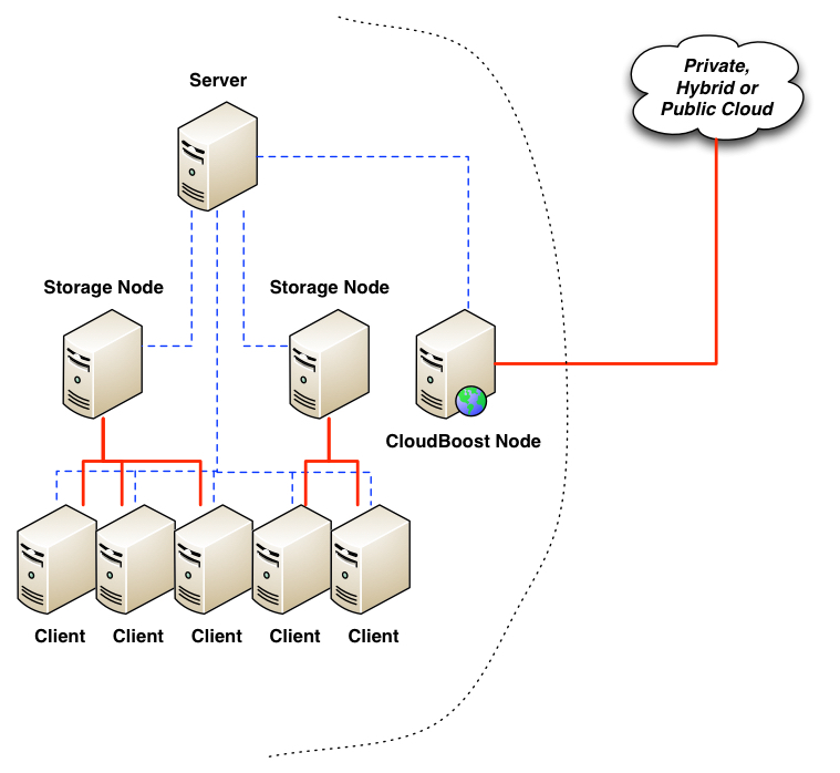
Introduced alongside NetWorker 8.2 SP1 is integration with a new EMC product, CloudBoost.

The purpose of CloudBoost is to allow a NetWorker server to write deduplicated backups from its datazone out to one of a number of different types of cloud (e.g., EMC ECS Storage Service, Google Cloud Storage, Azure Cloud Storage, Amazon S3, etc.) in an efficient form.

The integration point is quite straight forward, designed to simplify the configuration within NetWorker.

A CloudBoost system is a virtual appliance that can be deployed within your VMware vSphere environment. The appliance is an “all in one” system that includes:

NetWorker 8.2 SP1 storage node/client software
CloudBoost management console
CloudBoost discovery service

One of the nifty functions that CloudBoost performs in order to make deduplicated storage to the cloud efficient is a splitting of metadata and actual content. The metadata effectively relates to all the vital information the CloudBoost appliance has to know in order to access content from the object store it places in the selected cloud. While the metadata is backed up to the cloud, all metadata operations will happen against the local copy of the metadata, thereby significantly speeding up access and maintenance operations. (And everything written out to cloud is done so using AES-256 encryption, keeping it safe from prying eyes.)

A CloudBoost appliance can logically address 400TB of storage in the cloud pre-deduplication. With estimated deduplication ratios of up to 4x for data analysis performed by EMC, that might equate to up to 1.6PB of actual stored data, and it can be any data that NetWorker has backed up.

Once a CloudBoost appliance has been deployed (consisting of VM provisioning and connection to a supported cloud storage system), and integrated into NetWorker as storage node with in-built AFTD, getting long-term data out to the cloud is as simple as executing a clone operation against the required data, with the destination storage node being the CloudBoost storage node. Since the data is written to the CloudBoost embedded NetWorker Storage Node, recovery from backups that have been sent to the cloud is as simple as executing a recovery with the copy on the CloudBoost appliance being selected to use.

In other words, once it’s been setup, it’s business as usual for a NetWorker administrator or operator.

To get a thorough understanding of how CloudBoost and NetWorker integrate, I suggest you read the Release Notes and Integration Guide (you’ll need to log into the EMC support website to view those links). Additionally, there’s an excellent overview video you can watch here:

20 Jun 06:58

Pool size and deduplication

by Preston de Guise

When you start looking into deduplication, one of the things that becomes immediately apparent is … size matters. In particular, the size of your deduplication pool matters.

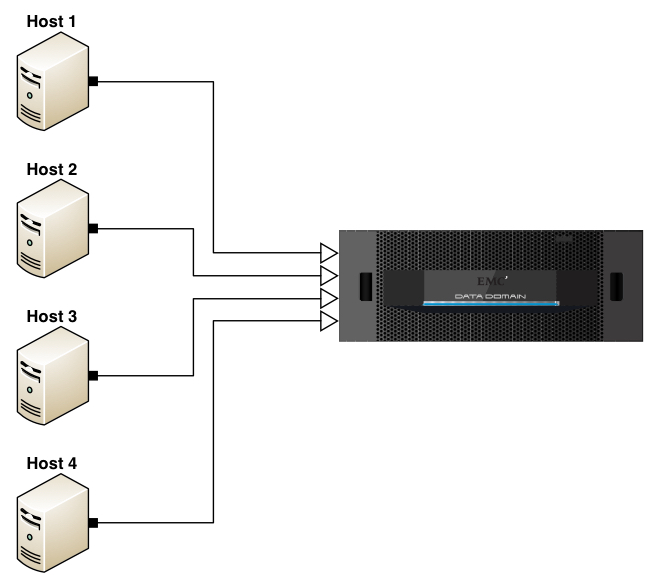
In this respect, what I’m referring to is the analysis pool for comparison when performing deduplication. If we’re only talking target based deduplication, that’s simple – it’s the size of the bucket you’re writing your backup to. However, the problems with a purely target based deduplication approach to data protection are network congestion and time wasted – a full backup of a 1TB fileserver will still see 1TB of data transferred over the network to have most of its data dropped as being duplicate. That’s an awful lot of packets going to /dev/null, and an awful lot of bandwidth wasted.

For example, consider the following diagram being of a solution using target only deduplication (e.g., VTL only or no Boost API on the hosts):

In this diagram, consider the outline arrow heads to indicate where deduplication is being evaluated. Thus, if each server had 1TB of storage to be backed up, then each server would send 1TB of storage over to the Data Domain to be backed up, with deduplication performed only at the target end. That’s not how deduplication has to work now, but it’s a reminder of where we were only a relatively short period of time ago.

That’s why source based deduplication (e.g., NetWorker Client Direct with a DDBoost enabled connection, or Data Domain Boost for Enterprise Applications) brings so many efficiencies to a data protection system. While there’ll be a touch more processing performed on the individual clients, that’ll be significantly outweighed by the ofttimes massive reduction in data sent onto the network for ingestion into the deduplication appliance.

So that might look more like:

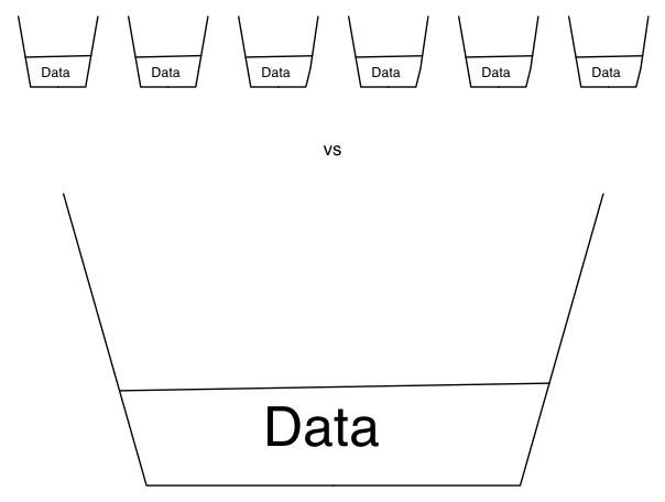
I.e., in this diagram with outline arrow heads indicating location of deduplication activities, we get an immediate change – each of those hosts will still have 1TB of backup to perform, but they’ll evaluate via hashing mechanisms whether or not that data actually needs to be sent to the target appliance.

There’s still efficiencies to be had even here though, which is where the original point about pool size becomes critical. To understand why, let’s look at the diagram a slightly different way:

In this case, we’ve still got source deduplication, but the merged lines represent something far more important … we’ve got global, source deduplication.

Or to put it a slightly different way:

Target deduplication:
- Client: “Hey, here’s all my data. Check to see what you want to store.”
Source deduplication (limited):
- Client: “Hey, I want to backup <data>. Tell me what I need to send based on what I’ve sent you before.”
Source deduplication (global):
- Client: “Hey, I want to backup <data>. Tell me what I need to send based on anything you’ve ever received before.”

That limited deduplication component may not be limited on a per host basis. Some products might deduplicate on a per host basis, while others might deduplicate based on particular pool sizes – e.g., xTB. But even so, there’s a huge difference between deduplicating against a small comparison set and deduplicating against a large comparison set.

Where that global deduplication pool size comes into play is the commonality of data that exists between hosts within an environment. Consider for instance the minimum recommended size for a Windows 2012 installation – 32GB. Now, assume you might get a 5:1 deduplication ratio on a Windows 2012 server (I literally picked a number out of the air as an example, not a fact) … that’ll mean a target occupied data size of 6.4GB to hold 32GB of data.

But we rarely consider a single server in isolation. Let’s expand this out to encompass 100 x Windows 2012 servers, each at 32GB in size. It’s here we see the importance of a large pool of data for deduplication analysis:

If that deduplication analysis were being performed at the per-server level, then realistically we’d be getting 100 x 6.4GB of target data, or 640GB.
If the deduplication analysis were being performed against all data previously deduplicated, then we’d assume that same 5:1 deduplication ratio for the first server backup, and then much higher deduplication ratios for each subsequent server backup, as they evaluate against previously stored data. So that might mean 1 x 5:1 + 99 x 20:1 … 164.8GB instead of 640GB or even (if we want to compare against tape) 3,200GB.

Throughout this article I’ve been using the term pool, but I’m not referring to NetWorker media pools – everything written to a Data Domain as an example, regardless of what media pool it’s associated with in NetWorker will be globally deduplicated against everything else on the Data Domain. But this does make a strong case for right-sizing your appliance, and in particular planning for more data to be stored on it than you would for a conventional disk ‘staging’ or ‘landing’ area. The old model – backup to disk, transfer to tape – was premised on having a disk landing zone big enough to accommodate your biggest backup, so long as you could subsequently transfer that to tape before your next backup. (Or some variant thereof.) A common mistake when evaluating deduplication is to think along similar lines. You don’t want storage that’s just big enough to hold a single big backup – you want it big enough to hold many backups so you can actually see the strategic and operational benefit of deduplication.

The net lesson is a simple one: size matters. The size of the deduplication pool, and what deduplication activities are compared against will make a significantly noticeable impact to how much space is occupied by your data protection activities, how long it takes to perform those activities, and what the impact of those activities are on your LAN or WAN.

20 Jun 06:58

Cloud is about startups and that’s not enough

by Keith Townsend

Former Netflix Architect Adrian Cockcraft and Speaking In Tech host Greg Knierieman had an interesting exchange on Twitter. Adrian compared Netflix’ $100M investment in House of Cards to Zynga’s $100 outlay in a data center. .@adrianco If you are going

20 Jun 06:57

Thinking Like a Data Scientist – Part II

by Bill Schmarzo

Bill Schmarzo

In “Thinking Like a Data Scientist – Part I”, we examined the challenges for getting the business users to think like data scientists when contemplating where and how to leverage big data to drive business value. We introduced a “Thinking Like a Data Scientist” process that starts with identifying and understanding the organization’s top-level strategic business initiatives, then uses a “Strategic Nouns” technique to create potential business questions that were descriptive, predictive or in nature.

We will now complete this exercise by introducing two additional techniques that we can use to uncover new variables or metrics that would be excellent predictors of business performance.

Thinking Like A Data Scientist Process (Continued)

Step 4: By Analysis. “By” Analysis is a technique for leveraging a business stakeholder’s natural question and query process to uncover:

Additional data sources
Additional dimensional entity characteristics
Additional areas for analytics exploration

“By” Analysis exploratory sentence format looks like the following:

“I want to see sales and product margin by product category, store, store remodel date, day of week, store demographics, and customer demographics”
“I want to trend hospital admissions by disease category, zip code, patient demographics, hospital size, area demographics and day of week“
“I want to compare current versus previous maintenance issues by turbine, turbine manufacturer, date installed, last maintenance date, maintenance person and weather conditions”

Check out my blog titled “Leverage By Analysis To Expand Your Data Science Perspectives” that covered the “By” Analysis in a bit more detail.

Figure 3 shows an example of “By” Analysis for a hypothetical Foot Locker merchandising example from the perspective of the customer. We asked the business users (in a facilitated brainstorming session) to brainstorm the different dimensions and/or attributes of the strategic noun upon which they were focused. You would do this same exercise for each of your strategic nouns.

Figure 3: Foot Locker “By” Analysis Example

The significant number and variety of “By” dimensions and attributes that can surface in a brainstorming session can lead to incredible insight. And remember as you go through this process, all ideas are worthy of consideration; this is not the point to try to filter the creative ideas or handcuff the creative thinking process!

Step 5: Score Technique. The purpose of the “Score” technique is to look for groupings of strategic noun dimensions and attributes that can be combined to create a more predictive and actionable score. These scores are critical components of our “thinking like a data scientist” process by supporting the decisions that we are trying to make, and/or what actions or outcomes are trying to predict with respect to our targeted business initiative.

Scores are very important constructs in the world of data science, and can help to cement the business stakeholders’ buy-in to the data science process. The best familiar score example might be the FICO[1] score, which combines a multiple questions and dimensions about a loan applicant’s finance history to create a single score that lenders use to predict a borrower’s ability to repay a loan (see Figure 4).

Figure 4: FICO Score Example

Scores can be created to provide predictive insights across a number of different industries and across a number of different business initiatives. Figure 5 shows some example scores from different industries.

Figure 5: Sample Scores Across Different Industries

So let’s build off of the variables and metrics that were uncovered in the “By” Analysis and see if we can integrate any of those variables or metrics into a higher-level score. In our Foot Locker example, we might want to group the Favorite sports, Favorite teams, High School sports and College sports into a score that measures that individuals “Sports Team Passion.” We might discover other potential scores around their level of current “Athletic Activity” (see Figure 6).

Figure 1: Foot Locker Predictive Scores

To be honest, this is probably the most enjoyable part of the process as you brainstorm additional data sources and metrics that can be used as part of your score. Again remember, no idea is a bad idea. Let the data science team decide via their analytic modeling which data sources and metrics are the best predictors of business performance.

Step 6: Close The Loop. The final step in the “Thinking Like A Data Scientist” exercise is “closing the loop” with respect to what analytics-driven scores or recommendations that we need to deliver to our key business stakeholders. You can use a simple “Recommendations Worksheet” that ties the decisions that our business stakeholders need to make (in support of the targeted business initiative) to the predictive and prescriptive analytics that we are going to need to build.

Last is the creation of the user-experience mockup that validates that we are building the right analytics and have a high-level understanding of where and how to deliver those scores and recommendations (e.g., management dashboards and reports, and operational systems such as the call center, procurement, sales, marketing, finance, etc.)

To get examples of these exercises, you’re going to have to enroll in my University of San Francisco “Big Data MBA” course. Sorry, got to save some homework for my students!!

Summary

Data scientists are critical to advanced analytics, and Ibelieve that you cannot have too many data scientists. But an important challenge is to get your business users to “think like a data scientist” when contemplating data sources and metrics that might be better predictors of business performance. Having a business organization that can “think like a data scientist” will drive better collaboration with your data science team and ultimately, lead to better predictive and prescriptive results, and… value to the business.

Okay Big Data MBA class, get ready for your next assignment!!

Thinking Like a Data Scientist – Part II
Bill Schmarzo

20 Jun 06:57

VMware’s classroom requirement for certification is still horrible

by Keith Townsend

I never understood why VMware requires you take a course to get certified for a technology as common as VMware vSphere. There might have been a time where it was needed. I imagine back when no one heard of x86

20 Jun 06:57

vShield Endpoint with vSphere 6.0

by Josh Townsend

I’ve heard some questions regarding vShield Endpoint being supported with vSphere 6.0. Some of the confusion has come from various announcements of End of Availability and End of Support for vCloud Networking and Security. Before I answer the question of using vShield Endpoint with vSphere 6.0, let’s first look at the history of the vShield product line to see where the confusion may come from. There has been many changes due to the rapid pace of innovation and developments in virtual networking and security:

May 2009: vShield Zones 1.0 released, providing an application-aware firewall built for VMware vCenter Server integration. vSphere 4.0 is the current version of vSphere. vSphere Advanced, Enterprise and Enterprise Plus editions are entitled to vShield Zones.
August 2010: VMware vShield 4.1 is released along with vSphere 4.1. vShield Edge, App and Endpoint are introduced and packaged with vShield Zones. All vShield components are managed by vShield Manager. vShield (Suite) is available as add-on licenses. vShield Zones remains a part of vSphere Enterprise and Enterprise Plus licensing.
July 2011: vShield Data Security is announced.
September 2011: VMware vShield 5.0 is released, along with vSphere 5.0. vShield 5.0 adds vShield Data Security capabilities. If you were running ESX 4.1 with vShield Zones 4.1, and wanted to upgrade to ESXi 5.0, you must manually uninstall vShield Manager 4.1 and Zones 4.1, upgrade to ESXi 5.0, then install vShield Manager 1.0 and Zones 1.0 that were released with vSphere 5.0. Yes, this is confusing at best…. vShield Endpoint is made available as part of the VMware View 4 Premier Edition bundle.
August 2012: vShield Zones 4.1 reaches End of Availability (EOA) and End of General Support (EOS). However, vShield Zones 1.0 that was released with vSphere 5.0 remains available for download through vSphere 5.1. The vShield Zones virtual firewall provided very basic segmentation and traffic filtering capabilities using the VMsafe API, which is deprecated (thus further investment for feature development or support can not be justified). VMware plans to continue to invest in vCloud Networking and Security, which covers the majority of use cases for vShield Zones.
July 2012: VMware acquires Nicira for $1.26 Billion. VMware NSX will eventually come from this acquisition.
August 2012: vShield Endpoint is now included in every vSphere Edition (except vSphere Essentials). The licensing change makes vShield Endpoint available for all customers, with an active SnS, running vSphere 5.1.x, vSphere 5.0.x, or vSphere 4.1 U3!
August 2012: vSphere 5.1 and vCloud Networking and Security (vCNS) 5.1 are announced. vCNS includes vShield Edge, App and Endpoint. vCNS is available as an add-on license to vSphere, and is included with vCloud Director. With the general availability of VMware vCloud Networking and Security 5.1 in September 2012, VMware announced an end of availability date of October 15, 2012 for the standalone vShield family of products (i.e, vShield Edge, vShield App, vShield Data Security and vShield Endpoint.) VMware will continue to support maintenance releases for the vShield products until September 1, 2013.
- vCloud Networking and Security is sold in two editions:
  - Standard Edition -‐ provides the following features: firewall, VPN, VXLAN, vCloud Ecosystem framework, Network Address Translation, and Dynamic Host Control Protocol.
  - Advanced Edition – Provides all the features of Standard Edition plus high availability, load balancing, and data security.

August 2012: vCloud Suite 5.1 is announced. This first iteration of the vCloud Suite bundled vSphere, vCloud Director, vCloud Connector, vFabric Application Director, vCloud Networking and Security 5.1, vCenter Operations Management Suite, vCenter Site Recovery Manager and vCloud Automation Center. VMware offered a $1 upgrade from vSphere Enterprise Plus to vCloud Suite Standard – customers who took advantage of this deal are now licensed for vCloud Networking and Security through the vCloud Suite.
- With vCloud Suite, VMware is now selling vCloud Networking and Security with two licensing options: bundled with the vCloud Suites and licensed per processor; or sold stand alone, and licensed per VM.
September 2013: vCloud Suite 5.5 is released. vCloud Suite 5.5 includes vCloud Networking and Security 5.5; vCloud Networking and Security 5.5 is only available as part of VMware vCloud Suite 5.5 and is not available as a standalone product. At the same time, VMware announced the End of Availability (“EOA”) of the VMware vCloud Networking and Security 5.1 Standard and Advanced editions for sale as standalone products effective September 30, 2013.
September 2013: VMware announces general availability of VMware NSX. NSX is a stand-alone product with some functionality that overlaps vCNS.
March 2015: vSphere 6.0 and vCloud Suite 6.0 are announced.
- vCloud Networking and Security is removed from the vCloud Suite bundle – this means that vCNS has reached End of Availability because it was only available through the vCloud Suite bundle. However, vCNS 5.5 remains supported through September 2016 for customers who were already licensed.
- NSX is not included in the vCloud Suite. vCloud Suite customers who are ready to take advantage of advanced software-defined networking and security services have the option to purchase NSX for vSphere at a reduced add-on price. NSX provides layer 2 to layer 7 network virtualization, with security policies that follow workloads across the data center for faster network provisioning and management.

And that brings us to today – At first glance, it would appear that all vShield and vCloud Networking and Security products are end of availability and not available for use with vSphere 6.0. vShield Manager, a component of vCNS, is needed to deploy and mange the vShield Endpoint agent on ESXi hosts, so customers began to question whether vShield Endpoint was licensed and compatible with vSphere 6.0 (and I suspect some of our security partners also began to wonder). So what’s the deal?

vShield Endpoint is supported with vSphere 6.0, and licensing is included in vSphere editions Essentials Plus and above! vCloud Networking and Security was updated to version 5.5.4.x to support vSphere 6.0. This VMware KB sheds a little light on this: Implementation of VMware vShield Endpoint beyond vCloud Networking and Security End of Availability (EOA) (2110078). Be sure to check the VMware Product Interoperability Matrixes to verify you have the supported version of vCNS for your version of vSphere (vCenter AND ESXi).

So how do you use vShield Endpoint with vSphere 6.0? vShield Endpoint requires vCNS (specifically, vShield Manager/vCloud Networking and Security Manager) for configuration and management. Any entitled customers will be able to download vCNS to obtain vCloud Networking and Security Manager. Sounds good, except that until very recently vCloud Networking and Security was not included in the vSphere 6.0 downloads (and it is still not listed under vSphere with Operations Management 6.0 downloads or vCloud Suite 6.0 downloads sections on http://my.vmware.com. If you don’t see vCloud Networking and Security in your product downloads on http://my.vmware.com use the search functionality in the downloads section to look for “vShield 5.5.4″. Note that as of today, the latest version is 5.5.4.1.

So what happens after vSphere 6.0? As far as I know, vCloud Networking and Security will not be available – features in NSX will replace vCNS/vShield features. NSX supports Guest Introspection. Guest Introspection strengthens security for virtual machines while improving performance for endpoint protection by offloading antivirus and anti-malware agent processing to a dedicated Security Virtual Appliance that is delivered and supported by VMware partners (such as Symantec, McAfee, TrendMicro). As of today, you have to acquire NSX licenses as add-on licensing to vCloud Suite or a la carte to your vSphere/vSOM environment (i.e. NSX is not included in vCloud Suite). I have no insight into whether vCloud Suite or NSX licensing will change for future versions.

Customers who choose to go the NSX path will be able to upgrade from vShield Endpoint 5.5 to vShield Endpoint 6.0 and use NSX Manager to perform administration and operations on vShield Endpoint (see this documentation for more: https://pubs.vmware.com/NSX-6/index.jsp#com.vmware.nsx.install.doc/GUID-45B09850-AB5A-4232-AE7C-6A80541A2AF0.html).

vShield Endpoint partner solutions will continue to be supported per this VMware KB article: Support for partner integrations with VMware vShield Endpoint and VMware vCloud Networking and Security (2105558)

Bottom line: vShield Endpoint is supported with vSphere 6.0, and licensing is included in vSphere editions Essentials Plus and above! Verify with your 3rd party security vendor that they support vCloud Networking and Security Manager v.5.5.4.x and vSphere 6.0. If so, upgrade vCloud Networking and Security Manager to v.5.5.4.x and then upgrade vSphere to version 6.0. Note that the official Update sequence for vSphere 6.0 and its compatible VMware products (2109760) has you upgrading vCenter and ESXi to 6.0 before vShield Endpoint to 5.5.4.x, but I don’t think it is correct (because vShield 5.5.3 and earlier do not support vSphere 6.x, but vShield 5.5.4.x supports vSphere 5.5 and earlier). Check with VMware Support, the VMware Product Interoperability Matrixes and, of course, test your upgrade in a lab. Hope this helps clear up any confusion.

The post vShield Endpoint with vSphere 6.0 appeared first on VMtoday.

20 Jun 06:56

Veeam & Data Domain: Advanced Setup and Replication

by Justin Paul

Recently while working with a customer we had to get a little creative with an installation and I thought I would share the experience. Here is a little background info… Datacenter and Hardware Layout: Customer has 2 datacenter: one on the east coast, one in the midwest Customer has vSphere clusters at both datacenters Customer […]

31 May 20:19

Like a Well-Oiled Machine

by Charles Robinson

It was Housekeeping Sunday in Dirk’s small IT shop, which usually meant taking their diminutive lot of servers down for routine maintenance. Dirk thought he’d change it up this week and add some actual cleaning to their housekeeping tasks. He knew just the man for the job too - Andrew, the Big Boss’s nephew.
Andrew couldn’t be trusted with much, but he was assigned to work with Dirk on this Housekeeping Sunday so he would have to be assigned a task he couldn’t possibly screw up. Several of the servers hadn’t been physically cleaned in a while and their dust bunnies had evolved in to full-blown Killer Rabbits of Caerbannog.

Dirk dispatched Andrew to the IT closet that doubled as the janitor’s storage room. “All the cleaning supplies you could possibly need are in there,” Dirk assured him. “Just use the cans of computer duster though. They should already have those little red straws jammed on to them and the label says ‘Electronics Duster’ in big letters. When you see dust, just point and shoot.”

“YES SIR!” Andrew shot back, with a sarcastic salute. Dirk brushed it off and went back to the remote firewall maintenance he was working on.

About half an hour later, Dirk’s phone buzzed on his desk with a text message from Andrew. “CAN U COME IN HERE?? Comps r broken.” It was immediately followed by a swarm of buzzes from email alerts about key servers not shutting down gracefully. Gravely concerned, Dirk rushed to the IT/Janitor closet in time to see Andrew stumble out of the room coughing and looking dazed.

“I don’t know what happened, man. I sprayed the stuff at the dust like you said, things started smoking, then the servers started crashing.” Andrew recounted.

“You should shut the servers down before you start opening them and spraying computer duster in there!” Dirk said, peering inside the closet. His nostrils were greeted with the scent of burning chemicals that were not native to cans of air. On the work bench he saw empty cans of WD–40 laying there, red straws and all.

“We should get some different cleaning junk, I don’t think that works right!” Andrew blurted out from behind him.

“For once, you’re right about something Andrew…” Dirk replied, as his head began to wrap around the fact that Housekeeping Sunday just became Disaster Control Sunday. But at least all the servers were now well-lubricated.

Ed. note: Someone (most specifically, me) did not get the next episode of TDWTF:Live! edited in time for this week. Our next episode, with John Lange, will appear next week. - Remy

[Advertisement] BuildMaster is more than just an automation tool: it brings together the people, process, and practices that allow teams to deliver software rapidly, reliably, and responsibly. And it's incredibly easy to get started; download now and use the built-in tutorials and wizards to get your builds and/or deploys automated!

Ronald.phillips likes this

31 May 20:17

CodeSOD: Sea of SQL

by Ellis Morning

Andy writes: “Operations reported that a query was taking a long time. Even the 'developers' of this query didn't know why it was taking a long time.”

I tell ya, folks… some submissions, you just set down and back away slowly… then hunt up a magnifying glass and a bottle of aspirin.


SELECT /*+ optimizer_features_enable('9.2.0') */ N1.ORDER_ID AS ORDER_ID, N1.N1_STATUS_ID AS N1_STATUS_ID, N1.SKU_ID AS SKU_ID, O.SITE_ID AS SITE_ID, O.ORDER_DT AS ORDER_DT, O.D_TOTAL_PRICE AS PRICE, RS.LEGAL_NAME AS RESELLER_LEGAL_NAME, PRS.LEGAL_NAME AS PARENT_RESELLER_LEGAL_NAME, S.COMPANY_NAME AS SITE_COMPANY_NAME, O.ORDER_STATE_ID AS ORDER_STATE_ID, ITEM.COUNTRY AS ITEM_COUNTRY, E.COUNTRY AS E_COUNTRY, C.CUST_SERVICE_REGION AS REGION, RS.PARTNER_LEVEL, O.FOLLOWUP_DT, N1.APPROVER_CONFIRM_DT, 'N' AS REISSUE_IND, sign(nvl(sum(distinct(R.ORDER_ID * ( -(SIGN(NVL(R.OVERRIDE_PERSON_ID, 0)) -1)) )), 0)) AS RSRC_CTRL_VIOLATION, max(decode( p.email_address, :1, 'Y', 'N' )) AS MANUAL_APPROVAL_IND, max(nvl(R.RESOURCE_CTRL_TYPE_ID, 0)) AS RESOURCE_CTRL_TYPE_ID , nvl(CFA.POLL_STATUS, 'N/A') AS POLL_STATUS , CFA.APPROVE_METHOD FROM ORDERS_N1 N1, ORDERS O, ENTERPRISE E, ENTERPRISE RS, ENTERPRISE PRS, SITE S, ORDERS_RSRC_CTRL R, PERSON P, COUNTRY C, SITE_ITEM ITEM , C ERT_FILE_APPROVE_DV_T CFA WHERE N1.ORDER_ID = O.ORDER_ID AND N1.N1_STATUS_ID  3 AND N1.N1_STATUS_ID  10 AND O.CUST_ENTERPRISE_ID = E.ENTERPRISE_ID AND O.RESELLER_ENTERPRISE_ID = RS.ENTERPRISE_ID AND RS.RESELLER_REFERRED_BY_ENT_ID = PRS.ENTERPRISE_ID AND O.SITE_ID = S.SITE_ID AND O.ORDER_ID = R.ORDER_ID(+) AND O.ORDER_COMPLETE_IND = 'N' AND O.ORDER_ID = ITEM.ORDER_ID AND ITEM.ITEM_ID = CFA.ITEM_ID (+) AND (ITEM.COUNTRY IS NOT NULL AND C.COUNTRY_CD = ITEM.COUNTRY OR ITEM.COUNTRY IS NULL AND C.COUNTRY_CD = E.COUNTRY) AND O.ORDER_DT >= to_date(:2, 'mmddyyyyhh24miss') AND O.ORDER_DT  220 GROUP BY N1.ORDER_ID, N1.N1_STATUS_ID, N1.SKU_ID, O.SITE_ID, O.ORDER_DT, O.D_TOTAL_PRICE, RS.LEGAL_NAME, PRS.LEGAL_NAME, S.COMPANY_NAME, O.ORDER_STATE_ID, ITEM.COUNTRY, E.COUNTRY, C.CUST_SERVICE_REGION, RS.PARTNER_LEVEL, O.FOLLOWUP_DT, N1.APPROVER_CONFIRM_DT, CFA.POLL_STATUS , CFA.APPROVE_METHOD UNION SELECT /*+ optimizer_features_enable('9.2.0') */ N1.ORDER_ID AS ORDER_ID, N1.N1_STATUS_ID AS N1_STATUS_ID, N1.SKU_ID AS SKU_ID, O.SITE_ID AS SITE_ID, O.ORDER_DT AS ORDER_DT, O.D_TOTAL_PRICE AS PRICE, RS.LEGAL_NAME AS RESELLER_LEGAL_NAME, PRS.LEGAL_NAME AS PARENT_RESELLER_LEGAL_NAME, S.COMPANY_NAME AS SITE_COMPANY_NAME, O.REISSUE_ORDER_STATE_ID AS ORDER_STATE_ID, ITEM.COUNTRY AS ITEM_COUNTRY, E.COUNTRY AS E_COUNTR Y, C.CUST_SERVICE_REGION AS REGION, RS.PARTNER_LEVEL, O.FOLLOWUP_DT, N1.APPROVER_CONFIRM_DT, 'Y' AS REISSUE_IND, sign(nvl(sum(distinct(R.ORDER_ID * ( -(SIGN(NVL(R.OVERRIDE_PERSON_ID, 0)) -1)) )), 0)) AS RSRC_CTRL_VIOLATION, max(decode( p.email_address, :5, 'Y', 'N' )) AS MANUAL_APPROVAL_IND, max(nvl(R.RESOURCE_CTRL_TYPE_ID, 0)) AS RESOURCE_CTRL_TYPE_ID , nvl(CFA.POLL_STATUS, 'N/A') AS POLL_STATUS , CFA.APPROVE_METHOD FROM ORDERS_N1 N1, ORDERS O, ENTERPRISE E, ENTERPRISE RS, ENTERPRISE PRS, SITE S, ORDERS_RSRC_CTRL R, PERSON P, COUNTRY C, SITE_ITEM ITEM , ITEM_FILE_APPROVE_DV_T CFA WHERE N1.ORDER_ID = O.ORDER_ID AND O.CUST_ENTERPRISE_ID = E.ENTERPRISE_ID AND O.RESELLER_ENTERPRISE_ID = RS.ENTERPRISE_ID AND RS.RESELLER_REFERRED_BY_ENT_ID = PRS.ENTERPRISE_ID AND O.SITE_ID = S.SITE_ID AND O.ORDER_ID = R.ORDER_ID(+) AND O.ORDER_ID = ITEM.ORDER_ID AND ITEM.ITEM_ID = CFA.ITEM_ID (+) AND ITEM.ITEM_STATUS_ID = 5 AND (ITEM.COUNTRY IS NOT NULL AND C.COUNTRY_CD = ITEM.COUNTRY OR C ERT.COUNTRY IS NULL AND C.COUNTRY_CD = E.COUNTRY) AND ITEM.START_DT >= to_date(:6, 'mmddyyyyhh24miss') AND ITEM.START_DT  220 GROUP BY N1.ORDER_ID, N1.N1_STATUS_ID, N1.SKU_ID, O.SITE_ID, O.ORDER_DT, O.D_TOTAL_PRICE, RS.LEGAL_NAME, PRS.LEGAL_NAME, S.COMPANY_NAME, O.REISSUE_ORDER_STATE_ID, ITEM.COUNTRY, E.COUNTRY, C.CUST_SERVICE_REGI ON, RS.PARTNER_LEVEL, O.FOLLOWUP_DT, N1.APPROVER_CONFIRM_DT, CFA.POLL_STATUS , CFA.APPROVE_METHOD ORDER BY N1_STATUS_ID, ORDER_DT DESC

[Advertisement] Use NuGet or npm? Check out ProGet, the easy-to-use package repository that lets you host and manage your own personal or enterprise-wide NuGet feeds and npm repositories. It's got an impressively-featured free edition, too!

31 May 20:00

Fetch once, write many times

by jamiet

As I’ve said before these days I’m spending time working on Hadoop rather than SQL Server and one of my colleagues today alerted me to a rather cool feature Of Hive (in a nutshell Hive is the technology that makes enables us to write SQL statements against Hadoop). Check this out:

Pretty cool, no? From a single tablescan I can summarise and insert into two destinations. Its the capability of a SSIS dataflow, but in SQL. If I ever make it back to the SQL Server world I’ll be requesting this feature in T-SQL pronto.

@Jamiet

31 May 19:59

Azure Data Lake

by James Serra

At the recent Microsoft Build Developer Conference, Executive Vice President Scott Guthrie announced the Azure Data Lake. It is a new flavor of Azure Storage which can handle streaming data (low latency, high volume, short updates), is geo-distributed, data-locality aware and allows individual files to be sized at petabyte scale.

Azure Data Lake is built to solve for restrictions found in traditional analytics infrastructure and realize the idea of a “data lake” – a single place to store every type of data in its native format with no fixed limits on account size or file size, high throughput to increase analytic performance and native integration with the Hadoop ecosystem.

I have previously blogged about the benefits of a data lake (here). To review, a data lake is an enterprise wide repository of every type of data collected in a single place prior to any formal definition of requirements or schema for the purposes of operational and exploratory analytics. Data lakes remove many of the restrictions constraining traditional analytics infrastructure like the pre-definition of schema, the cost of storing large datasets, and the propagation of different silos where data is located. Once captured in the data lake, different computational engines like Hadoop can be used to analyze and mine the raw data to discover new insights. Data Lakes can also act as a lower cost data preparation location prior to moving curated data into a data warehouse. In these cases, customers would load data into the data lake prior to defining any transformation logic.

Capabilities of the Azure Data Lake include:

HDFS for the cloud: Azure Data Lake is Microsoft’s implementation of a Hadoop File System compatible with HDFS that works with the Hadoop ecosystem including Azure HDInsight, Hortonworks, and Cloudera
Unlimited storage, petabyte files: Azure Data Lake has unbounded scale with no limits to how much data can be stored in a single account (Azure blobs have a 500TB limit per account). Azure Data Lake can also store very large files in the petabyte-range with immediate read/write access and high throughput (Azure blobs have a 5TB limit for individual files)
Optimized for massive throughput: Azure Data Lake is built for running large analytic systems that require massive throughput to query and analyze petabytes of data. You need only focus on the application logic and throughput can be tuned to meet the needs of the application
High frequency, low latency, read immediately: Azure Data Lake is built to handle high volumes of small writes at low latency making it optimized for near real-time scenarios like website analytics, Internet of Things (IoT), analytics from sensors, and others
Store data in its native format: Azure Data Lake is built as a distributed file store allowing you to store unstructured, semi-structured and structured data without transformation or schema definition. This allows you to store all of your data and analyze them in their native format
Integration with Azure Active Directory: Azure Data Lake is integrated with Azure Active Directory for identity and access management over all of your data
Automatically replicates your data – 3 copies within a single data center
Uses Azure AD for security
Up and running in a few clicks: no hardware to purchase or install or tune or maintain. Scale out on demand

Azure Data Lake can be addressed with Azure Storage APIs and it’s also compatible with the Hadoop Distributed File System (HDFS). That means the same range of Hadoop clusters can use it as PolyBase can use in reverse.

Answers to common questions:

What are the differences between Azure Data Lake and Azure Storage? In summary, this includes petabyte file sizes, high throughput, and built-in Hadoop integration. Azure Storage is a generic store for many use cases whereas Azure Data Lake is optimized for doing big data analytics.

Will Azure Data Lake integrate with Azure HDInsight? Yes, Azure HDInsight will be able to access Azure Data Lake as a data source similar to how it accesses Azure Blobs today. This is available immediately at public preview allowing HDInsight customers to leverage a hyper scale big data repository in conjunction with Hadoop.

How is Azure Data Lake different from HDFS? Azure Data Lake is an implementation of HDFS in the cloud and leverages the WebHDFS REST interface. WebHDFS Rest APIs have a subset of the APIs available for HDFS.

When is Microsoft Azure Data Lake available? Today, Azure Data Lake is only available as a private preview. Public preview will be available post-Build conference. At public preview, Data Lake will be available at US East 2 data center.

What technologies can use the Azure Data Lake? Any HDFS compliant projects can use azure data lake (Spark, Storm, Flume, Sqoop, Kafka, R, etc). The idea is to put all your data in the Azure Data Lake and then later use any technology on top of it (Azure ML, Azure Data Factory, HDInsights, Azure Stream Analytics, DocumentDB, Hortonworks, Cloudera, Azure Event Hubs, Qubole, etc).

Couldn’t this be done before with Azure blob storage? The data lake is dramatically different that azure blog storage in a few areas. It is built specifically to run massive parallel queries, with a large improvement in throughput performance and scale and the ability to store large files. Also there is much bigger vision for the data lake and it will continue to differentiate more and more over blob storage.

You can sign up to be notified when the Azure Data Lake preview becomes available.

More info:

Microsoft BUILDs its cloud Big Data story

Azure Data Lake: Why you might want one

Microsoft Announces Azure SQL Database elastic database, Azure SQL Data Warehouse, Azure Data Lake

6 Key Features from Microsoft’s Azure Data Lake

Azure Data Lakes

31 May 19:59

Improving Partition Maintenance with Incremental Statistics

by Erin Stellato

SQL Server 2014 brought many new features that DBAs and developers looked forward to testing and using in their environments, such as the updatable clustered Columnstore index, Delayed Durability, and Buffer Pool Extensions. A feature not often discussed is incremental statistics. Unless you use partitioning, this isn’t a feature you can implement. But if you do have partitioned tables in your database, incremental statistics might have been something you were eagerly anticipating.

Note: Benjamin Nevarez covered some basics related to incremental statistics in his February 2014 post, SQL Server 2014 Incremental Statistics. And while not much has changed in how this feature works since his post and the April 2014 release, it seemed a good time to dig into how enabling incremental statistics can help with maintenance performance.

Incremental statistics are sometimes called partition-level statistics, and this is because for the first time, SQL Server can automatically create statistics that are specific to a partition. One of the previous challenges with partitioning was that, even though you could have 1 to n partitions for a table, there was only one (1) statistic which represented the data distribution across all of those partitions. You could create filtered statistics for the partitioned table – one statistic for each partition – to provide the query optimizer with better information about the distribution of data. But this was a manual process, and required a script to automatically create them for each new partition.

In SQL Server 2014, you use the STATISTICS_INCREMENTAL option to have SQL Server create those partition-level statistics automatically. However, these statistics are not used as you might think.

I mentioned previously that, prior to 2014, you could create filtered statistics to give the optimizer better information about the partitions. Those incremental statistics? They aren’t currently used by the optimizer. The query optimizer still just uses the main histogram that represents the entire table. (Post to come which will demonstrate this!)

So what’s the point of incremental statistics? If you assume that only data in the most recent partition is changing, then ideally you only update statistics for that partition. You can do this now with incremental statistics – and what happens is that information is then merged back into the main histogram. The histogram for the entire table will update without having to read through the entire table to update statistics, and this can help with performance of your maintenance tasks.

Setup

We’ll start with creating a partition function and scheme, and then a new table which we will partition. Note that I created a filegroup for each partition function as you might in a production environment. You can create the partition scheme on the same filegroup (e.g. PRIMARY) if you cannot easily drop your test database. Each filegroup is also a few GB in size, as we’re going to add almost 400 million rows.

USE [AdventureWorks2014_Partition];
GO
 
/* add filesgroups */
ALTER DATABASE [AdventureWorks2014_Partition] ADD FILEGROUP [FG2011];
ALTER DATABASE [AdventureWorks2014_Partition] ADD FILEGROUP [FG2012];
ALTER DATABASE [AdventureWorks2014_Partition] ADD FILEGROUP [FG2013];
ALTER DATABASE [AdventureWorks2014_Partition] ADD FILEGROUP [FG2014];
ALTER DATABASE [AdventureWorks2014_Partition] ADD FILEGROUP [FG2015];
 
/* add files */
ALTER DATABASE [AdventureWorks2014_Partition] ADD FILE 
( 
  FILENAME = N'C:\Databases\AdventureWorks2014_Partition\2011.ndf',
  NAME = N'2011', SIZE = 1024MB, MAXSIZE = 4096MB, FILEGROWTH = 512MB
) TO FILEGROUP [FG2011];
 
ALTER DATABASE [AdventureWorks2014_Partition] ADD FILE 
(
  FILENAME = N'C:\Databases\AdventureWorks2014_Partition\2012.ndf',
  NAME = N'2012', SIZE = 512MB, MAXSIZE = 2048MB, FILEGROWTH = 512MB
) TO FILEGROUP [FG2012];
 
ALTER DATABASE [AdventureWorks2014_Partition] ADD FILE 
(
  FILENAME = N'C:\Databases\AdventureWorks2014_Partition\2013.ndf',
  NAME = N'2013', SIZE = 2048MB, MAXSIZE = 4096MB, FILEGROWTH = 512MB
) TO FILEGROUP [FG2013];
 
ALTER DATABASE [AdventureWorks2014_Partition] ADD FILE
(
  FILENAME = N'C:\Databases\AdventureWorks2014_Partition\2014.ndf',
  NAME = N'2014', SIZE = 2048MB, MAXSIZE = 4096MB, FILEGROWTH = 512MB
) TO FILEGROUP [FG2014];
 
ALTER DATABASE [AdventureWorks2014_Partition] ADD FILE 
(
  FILENAME = N'C:\Databases\AdventureWorks2014_Partition\2015.ndf',
  NAME = N'2015', SIZE = 2048MB, MAXSIZE = 4096MB, FILEGROWTH = 512MB
) TO FILEGROUP [FG2015];
 
/* create partition function */
CREATE PARTITION FUNCTION [OrderDateRangePFN] ([datetime])
AS RANGE RIGHT FOR VALUES 
(
  '20110101',  -- everything in 2011
  '20120101',  -- everything in 2012
  '20130101',  -- everything in 2013
  '20140101',  -- everything in 2014
  '20150101'   -- everything in 2015
);
GO
 
/* create partition scheme */
CREATE PARTITION SCHEME [OrderDateRangePScheme]
AS PARTITION [OrderDateRangePFN] TO
  ([PRIMARY], [FG2011], [FG2012], [FG2013], [FG2014], [FG2015]);
GO
 
/* create the table */
CREATE TABLE [dbo].[Orders]
(
 [PurchaseOrderID] [int] NOT NULL,
 [EmployeeID] [int] NULL,
 [VendorID] [int] NULL,
 [TaxAmt] [money] NULL,
 [Freight] [money] NULL,
 [SubTotal] [money] NULL,
 [Status] [tinyint] NOT NULL,
 [RevisionNumber] [tinyint] NULL,
 [ModifiedDate] [datetime] NULL,
 [ShipMethodID] [tinyint] NULL,
 [ShipDate] [datetime] NOT NULL,
 [OrderDate] [datetime] NOT NULL,
 [TotalDue] [money] NULL
) ON [OrderDateRangePScheme] (OrderDate);

Before we add the data, we’ll create the clustered index, and note that the syntax includes the WITH (STATISTICS_INCREMENTAL = ON) option:

/* add the clustered index and enable incremental stats */
ALTER TABLE [dbo].[Orders] ADD CONSTRAINT [OrdersPK]
PRIMARY KEY CLUSTERED 
(
 [OrderDate],
 [PurchaseOrderID]
)
WITH (STATISTICS_INCREMENTAL = ON)
ON [OrderDateRangePScheme] ([OrderDate]);

What’s interesting to note here is that if you look at the ALTER TABLE entry in MSDN, it does not include this option. You will only find it in the ALTER INDEX entry… but this works. If you want to follow the documentation to the letter, you would run:

/* add the clustered index and enable incremental stats */
ALTER TABLE [dbo].[Orders]
ADD CONSTRAINT [OrdersPK]
PRIMARY KEY CLUSTERED 
(
 [OrderDate],
 [PurchaseOrderID]
) 
ON [OrderDateRangePScheme] ([OrderDate]);
GO
 
ALTER INDEX [OrdersPK] ON [dbo].[Orders] REBUILD WITH (STATISTICS_INCREMENTAL = ON);

Once the clustered index has been created for the partition scheme, we’ll load in our data and then check to see how many rows exist per partition (note this takes over 7 minutes on my laptop, you may want to add fewer rows depending on how much storage (and time) you have available):

/* load some data */
SET NOCOUNT ON;
DECLARE @Loops SMALLINT = 0;
DECLARE @Increment INT = 5000;
 
WHILE @Loops < 10000 -- adjust this to increase or decrease the number 
                     -- of rows in the table, 10000 = 40 millon rows
BEGIN
  INSERT [dbo].[Orders]
  ( [PurchaseOrderID]
   ,[EmployeeID]
   ,[VendorID]
   ,[TaxAmt]
   ,[Freight]
   ,[SubTotal]
   ,[Status]
   ,[RevisionNumber]
   ,[ModifiedDate]
   ,[ShipMethodID]
   ,[ShipDate]
   ,[OrderDate]
   ,[TotalDue] 
  )
  SELECT 
     [PurchaseOrderID] + @Increment
   , [EmployeeID]
   , [VendorID]
   , [TaxAmt]
   , [Freight]
   , [SubTotal]
   , [Status]
   , [RevisionNumber]
   , [ModifiedDate]
   , [ShipMethodID]
   , [ShipDate]
   , [OrderDate]
   , [TotalDue]
  FROM [Purchasing].[PurchaseOrderHeader];
 
  CHECKPOINT;
 
  SET @Loops = @Loops + 1;
  SET @Increment = @Increment + 5000;
END
 
/* Check to see how much data exists per partition */
SELECT
  $PARTITION.[OrderDateRangePFN]([o].[OrderDate]) AS [Partition Number]
  , MIN([o].[OrderDate]) AS [Min_Order_Date]
  , MAX([o].[OrderDate]) AS [Max_Order_Date]
  , COUNT(*) AS [Rows In Partition]
FROM [dbo].[Orders] AS [o]
GROUP BY $PARTITION.[OrderDateRangePFN]([o].[OrderDate])
ORDER BY [Partition Number];

Data per partition

We’ve added data for 2012 through 2015, with significantly more data in 2014 and 2015. Let’s see what our statistics look like:

DBCC SHOW_STATISTICS ('dbo.Orders',[OrdersPK]);

DBCC SHOW_STATISTICS output for dbo.Orders (click to enlarge)

With the default DBCC SHOW_STATISTICS command, we don’t have any information about statistics at the partition level. Fear not; we are not completely doomed – there is an undocumented dynamic management function, sys.dm_db_stats_properties_internal. Remember that undocumented means it is not supported (there is no MSDN entry for the DMF), and that it can change at any time without any warning from Microsoft. That said, it’s a decent start for getting an idea of what exists for our incremental statistics:

SELECT *
  FROM [sys].[dm_db_stats_properties_internal](OBJECT_ID('dbo.Orders'),1)
  ORDER BY [node_id];

Histogram information from dm_db_stats_properties_internal (click to enlarge)

This is a lot more interesting. Here we can see proof that partition-level statistics (and more) exist. Because this DMF is not documented, we have to do some interpretation. For today, we’ll focus on the first seven rows in the output, where the first row represents the histogram for the entire table (note the rows value of 40 million), and the subsequent rows represent the histograms for each partition. Unfortunately, the partition_number value in this histogram does not line up with the partition number from sys.dm_db_index_physical_stats for right-based partitioning (it does correlate properly for left-based partitioning). Also note that this output also includes the last_updated and modification_counter columns, which are helpful when troubleshooting, and it can be used to develop maintenance scripts that intelligently update statistics based on age or row modifications.

Minimizing maintenance required

The primary value of incremental statistics at this time is the ability to update statistics for a partition and have those merge into the table-level histogram, without having to update the statistic for the entire table (and therefore read through the entire table). To see this in action, let’s first update statistics for the partition which holds the 2015 data, partition 5, and we’ll record the time taken and snapshot the sys.dm_io_virtual_file_stats DMF before and after to see how much I/O occurs:

SET STATISTICS TIME ON;
 
SELECT 
  fs.database_id, fs.file_id, mf.name, mf.physical_name, 
  fs.num_of_bytes_read, fs.num_of_bytes_written
INTO #FirstCapture
FROM sys.dm_io_virtual_file_stats(DB_ID(), NULL) AS fs
INNER JOIN sys.master_files AS mf 
ON fs.database_id = mf.database_id 
AND fs.file_id = mf.file_id;
 
UPDATE STATISTICS [dbo].[Orders]([OrdersPK]) WITH RESAMPLE ON PARTITIONS(6);
GO
 
SELECT 
  fs.database_id, fs.file_id, mf.name, mf.physical_name, 
  fs.num_of_bytes_read, fs.num_of_bytes_written
INTO #SecondCapture
FROM sys.dm_io_virtual_file_stats(DB_ID(), NULL) AS fs
INNER JOIN sys.master_files AS mf 
ON fs.database_id = mf.database_id 
AND fs.file_id = mf.file_id;
 
SELECT f.file_id, f.name, f.physical_name, 
  (s.num_of_bytes_read - f.num_of_bytes_read)/1024 MB_Read,   
  (s.num_of_bytes_written - f.num_of_bytes_written)/1024 MB_Written
FROM #FirstCapture AS f
INNER JOIN #SecondCapture AS s 
ON f.database_id = s.database_id 
AND f.file_id = s.file_id;

Output:

SQL Server Execution Times:
CPU time = 203 ms, elapsed time = 240 ms.

File_stats data after updating one partition

If we look at the sys.dm_db_stats_properties_internal output, we see that last_updated changed for both the 2015 histogram and the table-level histogram (as well as a few other nodes, which is for later investigation):

Updated histogram information from dm_db_stats_properties_internal

Now we’ll update statistics with a FULLSCAN for the table, and we’ll snapshot file_stats before and after again:

SET STATISTICS TIME ON;
 
SELECT 
  fs.database_id, fs.file_id, mf.name, mf.physical_name, 
  fs.num_of_bytes_read, fs.num_of_bytes_written
INTO #FirstCapture2
FROM sys.dm_io_virtual_file_stats(DB_ID(), NULL) AS fs
INNER JOIN sys.master_files AS mf 
ON fs.database_id = mf.database_id 
AND fs.file_id = mf.file_id;
 
UPDATE STATISTICS [dbo].[Orders]([OrdersPK]) WITH FULLSCAN
 
SELECT 
  fs.database_id, fs.file_id, mf.name, mf.physical_name, 
  fs.num_of_bytes_read, fs.num_of_bytes_written
INTO #SecondCapture2
FROM sys.dm_io_virtual_file_stats(DB_ID(), NULL) AS fs
INNER JOIN sys.master_files AS mf 
ON fs.database_id = mf.database_id 
AND fs.file_id = mf.file_id;
 
SELECT 
  f.file_id, f.name, f.physical_name, 
  (s.num_of_bytes_read - f.num_of_bytes_read)/1024 MB_Read,   
  (s.num_of_bytes_written - f.num_of_bytes_written)/1024 MB_Written
FROM #FirstCapture2 AS f
INNER JOIN #SecondCapture2 AS s 
ON f.database_id = s.database_id 
AND f.file_id = s.file_id;

Output:

SQL Server Execution Times:
CPU time = 12720 ms, elapsed time = 13646 ms

Filestats data after updating with a fullscan

The update took significantly longer (13 seconds versus a couple hundred milliseconds) and generated a lot more I/O. If we check sys.dm_db_stats_properties_internal again, we find that last_updated changed for all the histograms:

Histogram information from dm_db_stats_properties_internal after a fullscan

Summary

While incremental statistics are not yet used by the query optimizer to provide information about each partition, they do provide a performance benefit when managing statistics for partitioned tables. If statistics only need to be updated for select partitions, just those can be updated. The new information is then merged into the table-level histogram, providing the optimizer more current information, without the cost of reading the entire table. Going forward, we hope that those partition-level statistics will be used by the optimizer. Stay tuned…

The post Improving Partition Maintenance with Incremental Statistics appeared first on SQLPerformance.com.

31 May 19:59

How would indexes on AG readable secondaries work?

Last weekend there was a suggestion on the MVP distribution list about having temporary nonclustered indexes on AG readable secondaries, in the same way that you can have temporary statistics on them. I replied that in my opinion it would be extremely difficult to do that, and said I’d blog about why. Here’s my explanation. Note that this isn’t an exhaustive list of all the problems, just the major ones that I see.

Where to store them?

There are several options that spring to mind for how to store these temporary indexes, with varying degrees of difficulty:

Automatically create a temporary filegroup on the readable secondary
1. This option has the problem that the readable secondary is read-only, and adding a filegroup would mean adding entries in a bunch of system tables (including sys.sysfiles1, sys.sysdbfiles, sys.sysbrickfiles, sys.sysprufiles). Even if this problem could be surmounted, there’s still the problem of…
2. The readable secondary is read-only, so where to store all the information about the indexes themselves? There are a large number of system tables that have information about an index (including sys.sysallocunits, sys.sysrowsets, sys.sysrscols, sys.sysidxstats, sys.sysiscols). Even if this problem could be surmounted, there’s still the problem of maintaining the index (see below).
Create an empty filegroup on the primary replica so there’s an empty filegroup to use on the readable secondary
1. This only solves 1.a above.
Store them in tempdb, the same as the temporary statistics
1. This solves 1.a and 1.b, but then has the added difficulty of…
2. Keeping track of the fact that there are indexes in tempdb that are really for another database, which already happens for temporary statistics, so that’s doable but there’s the much more complex problem of…
3. Making the Storage Engine (specifically the Access Methods) get data from the tempdb index instead of an index in the real database. That’s not a code change in the Storage Engine (because the Access Methods just creates and uses a data set over whatever the Query Processor asks it to), but the query plan will have to know that the index it’s referencing which purports to be on a table in the real database is actually in tempdb, so it asks the Storage Engine to read from the correct place. I can imagine this being quite a challenge for things like a key lookup based on a nonclustered index seek/scan.
4. This is the only potentially practical solution in my mind for where to create the temporary indexes.

That’s the easier part taken care of.

How to maintain them?

Assuming they are stored as in #3 above, then there’s the really hard problem of how to maintain the indexes, to keep them up-to-date with the underlying table (i.e. when an INSERT, UPDATE, or DELETE happens, make sure that all nonclustered indexes are updated accordingly). Creating the index would be relatively trivial using an online index build-like method, so I won’t go into that.

Back in SQL Server 2000, it would be much easier (although there weren’t any AGs back then :-) because the Storage Engine was responsible for real-time maintenance of nonclustered indexes. Since SQL Server 2005, however, this has been the purview of the Query Processor, so it drives maintaining indexes and the Storage Engine just does what it’s asked (insert a record here, update this column, etc.). There is functionality available to the Storage Engine to ask the Query Processor to manipulate nonclustered indexes without an operation occurring on the table – DBCC CHECKDB uses it for fixing missing or extra records in nonclustered indexes during repair operations.

Here’s the major problem with temporary indexes: the only data coming from the primary replica are physical log records. How to translate those physical log records into nonclustered index maintenance operations?

The only log records that are interesting are those related to the table itself (i.e. changes to the heap or clustered index). But log records are replayed by the recovery portion of the Storage Engine, not the Access Methods, so in the recovery portion, there is no context at all about the table, it’s columns, indexes, and so on. To make this work, the following would be required:

The recovery portion would have to know that the log records LOP_INSERT_ROWS, LOP_DELETE_ROWS, LOP_MODIFY_ROW, LOP_MODIFY_COLUMNS, plus anything else like truncating the table, changing from a heap to a clustered index and vice versa, for certain allocation units (i.e. those for any table with a temporary nonclustered index) need to be passed to a new piece of code to do the temporary index maintenance.
The new piece of code would have to know about the new indexes and do the index maintenance. In other words, Storage Engine nonclustered index maintenance like in SQL Server 2000 would have to be built again. There’s a complication with table record modifications, as the LOP_MODIFY_ROW and LOP_MODIFY_COLUMNS log records don’t say which columns are changing – just the offset and length of the change (they’re physical log records remember). The log record could potentially be changed to have a bitmap of column IDs being changed, that’s only present when there’s a temporary index on a readable secondary. More conditional code.
Another option is for the Query Processor on the primary replica to know that there’s a temporary index and generate special logical operation log records to aid in the maintenance of the index on the readable secondary (in the same way that transactional replication works). I think this would be easier than having to interpret regular log records and figure out what to do.
All this new code to be executed would potentially slow down the replay of log records, with the slow down increasing with each temporary index that’s added.

Summary

To summarize, there are possible solutions to how to store the temporary indexes and how to maintain them, but it’s a lot of tricky work and involves a big change to the recovery code, which is always fraught with danger as it’s such a critical portion of the Storage Engine. And I haven’t touched on partitioning, rebuild/reorganize, and other things you can do with indexes.

IMHO, the easiest solution is to not use temporary indexes and just create the indexes on the primary replica that you want to be there on the readable secondary. This doesn’t require any code changes and is available today. Of course there’s the potential downside of extra space being taken up, extra logging, and extra time to send that log to the secondaries, but I think this is the way to go.

Hope you found this interesting!

The post How would indexes on AG readable secondaries work? appeared first on Paul S. Randal.

31 May 19:59

Latest MVA Offerings for SQL Server and for Windows 10 (Yes it’s time to start looking at this)

by Greg Low

The team at Microsoft Virtual Academy (MVA) have pushed out some new content that’s relevant to database people.

First, if you’re wondering about using Azure for SQL Server, the Jumpstart for SQL Server in Azure VMs is worth a look. Longer term, I suspect we’ll mostly end up using SQL Server as a platform service (Azure SQL DB) but in the short-term, implementing it in a VM will be more common as it’s probably both easier when migrating existing applications and a little more familiar to most.

Next, if you have to deal with other databases (shock horror, yes there are others including open source ones), there is a course on Open Source Databases on Azure.

Finally, you would have to have been living under a rock not to notice that Windows 10 is coming. But now, it’s time to start to get your head around what’s different. There’s a course that covers off the Fundamentals of the Technical Preview of Windows 10.

Scott Weigand likes this

23 May 05:31

SQL Server Page Life Expectancy (PLE)

by psssql

This week I was involved in a conversation with Paul Randal relating to PLE per node vs PLE server wide.

There is an all-up PLE counter as well as individual, per NUMA node PLE counters. SQL Server Books Online describes the values as:

SQL Server Buffer Manager \ Page life expectancy – Indicates the number of seconds a page will stay in buffer pool without references.

SQL Server Buffer Node \ Page life expectancy – Indicates the minimum number of seconds a page will stay in buffer pool on this node without references.

The descriptions leave a bit to the imagination. It is pretty common place to ask someone about the all-up value and the assumption is a simple average of the individual node values. For example, using the following 4 Node values, the AVG = 1750 divided by 1000 = 175.

1000

2000

1500

2500

This is not the calculation used for all-up number. The Buffer Manager value is an average of the rates or the (Harmonic Mean.) Using the harmonic mean, run rates average, for this example the PLE = 155.

Paul outlines additional calculations and highlights the need to watch per node values for better management of your PLE targets in his post: http://www.sqlskills.com/blogs/paul/page-life-expectancy-isnt-what-you-think

Bob Dorr - Principal SQL Server Escalation Engineer

23 May 04:49

SQL Server 2014 Service Pack 1 is available (again)!

by Damian

I just got notified that the SQL Server 2014 SP1 is available for download. I was a part of "testing team" of this new / updated SP1 and found no issues! Hope you will not found them, too

Below you can find the official information about the SP1:

As previously communicated, the Service Pack 1 release on April 15 was recalled very shortly after going live on the Microsoft Download Center (only) to address a recall issue. That issue has been resolved, and after complete recertification is now available. The new release is v12.0.4100.1, KB3058865.

Approximately one year ago, we launched SQL Server 2014. Today, May 15, we are pleased to announce the release of SQL Server 2014 Service Pack 1 (SP1). The Service Pack is initially available for download on the Microsoft Download Center. SQL Server 2014 SP1 will be rolling out to additional venues including MSDN/TechNet, the Volume Licensing center, and Microsoft Update starting May 21, 2015.

SQL Server 2014 SP1 contains fixes provided in SQL Server 2014 CU 1 up to and including CU 5, as well as a rollup of fixes previously shipped in SQL Server 2012 SP2. For highlights of the release, please read the Knowledge Base Article for Microsoft SQL Server 2014 SP1.

As part of our continued commitment to software excellence for our customers, this upgrade is available to all customers with existing SQL Server 2014 deployments via the download links below.

http://www.microsoft.com/en-us/download/details.aspx?id=4669…
http://www.microsoft.com/en-us/download/details.aspx?id=4669…
http://www.microsoft.com/en-us/download/details.aspx?id=4669…

Cheers

Damian

Scott Weigand likes this

23 May 04:49

Continuous delivery and Azure SQL Database achieving the impossible

by simonsabin

I was very proud to be asked to speak at Ignite at the start of May. http://ignite.microsoft.com/speaker/speakermoreinfo/?speakerid=f0dfadd0-2498-e411-b87f-00155d5066d7 . I encounter much scepticism about continuous delivery for databases, more over many...(read more)

23 May 01:44

Big data needs a big cloud

by SQL Server Team

Brian Mitchell, Microsoft Senior Business Program Manager, took the stage at Ignite two weeks ago to discuss Planning Your Big Data Architecture on Azure. “Big Data” requires big scale. Mitchell covered how this is accomplished through storage strategies, partitioning, fault tolerance, and the right architecture to scale to the extremes of big data. If you want to explore cloud-based big data apps, be sure to check it out.

Ignite covered the cloud in depth. Make sure to take a look at all the other on-demand presentations, demos, and more.

23 May 01:44

New Article: Row Level Security for SQL

by RickHeiges

Recently, Tech Target was nice enough to ask me to start writing a series of articles for their SearchSQLServer.com website. I have often made good use of articles on their family of websites. I hope that the articles that I compose will prove helpful as well. I chose Row Level Security(RLS) for my first article for several reasons. First, I think it makes sense that an organization wants to maintain control as much as possible over the data it possesses. Now that I work for DB Best, Migrations from...(read more)

23 May 01:44

SQL Server 2016 public preview arriving this summer

by James Serra

SQL Server 2016 was recently announced. Top new features include:

Always Encrypted protects data at rest and in motion. With Always Encrypted, SQL Server can perform operations on encrypted data and best of all, the encryption key resides with the application in the customers trusted environment. Encryption and decryption of data happens transparently inside the application which minimizes the changes that have to be made to existing applications.
Stretch Database allows you to dynamically stretch your warm and cold transactional data to Microsoft Azure, so your operational data is always at hand, no matter the size, and you benefit from the low cost of using Microsoft Azure. You can use Always Encrypted with Stretch Database to extend your data in a more secure manner for greater peace of mind
Real-time Operational Analytics & In-Memory: OLTP For In-Memory OLTP, which customers today are using for up to 30x faster transactions than disk based systems, you will now be able to apply this technology tuned for transactional performance to a significantly greater number of applications as well as benefit from increased concurrency. With these enhancements, you also have the unique capability to use in-memory columnstore delivering 100X faster queries with in-memory OLTP for in-memory performance and real-time operational analytics
Built-in Advanced Analytics, PolyBase and Mobile BI deliver advanced analytics as an additional workload in SQL Server with proven technology from Revolution Analytics. Advanced analytics is more accessible and has increased performance for your advanced analytic workloads by bringing R processing closer to the data and building advanced analytic capabilities right into SQL Server. Additionally, Microsoft has built PolyBase into SQL Server, expanding the power to extract value from unstructured and structured data using your existing T-SQL skills.
Additional security enhancements for Row-level Security and Dynamic Data Masking
Improvements to AlwaysOn for more robust availability and disaster recovery with multiple synchronous replicas and secondary load balancing
Native JSON support to offer better performance and support for your many types of your data
SQL Server Enterprise Information Management (EIM) tools and Analysis Services get an upgrade in performance, usability and scalability
Faster hybrid backups, high availability and disaster recovery scenarios to backup and restore your on-premises databases to Azure and place your SQL Server AlwaysOn secondaries in Azure

Check out the data sheet for more details. You can sign up to be notified of the preview availability this summer

More info:

SQL Server 2016 public preview coming this summer

‘Always Encrypted’ Leads New SQL Server 2016 Features

SQL Server 2016 is coming….

Reading the SQL Server 2016 Data Sheet

Video on new SQL Server 2016 features: The SQL Server Evolution and The SQL Server Evolution: Deep Dive

SQL Server 2016 Security Roadmap Session Notes #MSIgnite

SQL Server 2016

Microsoft Breathes Life back into SQL Server BI On-Prem

Top 7 Features Coming to SQL Server 2016

23 May 01:44

Availability Groups and Columnstore Indexes

This week Paul, Kimberly, Erin, and Tim are at SQLIntersection in Arizona presenting, and one of the best things about presenting at conferences is the questions that get asked about SQL Server features. Kimberly was asked a question about whether or not columnstore indexes could be used in a database that participates in an Availability Group or not and there is conflicting information available online. Since I have multiple 2012 and 2014 Availability Groups setup in my laptop for teaching our Immersion Events, I spent a little time testing and agreed to blog about the findings.

Columnstore indexes can be created in any database participating in an Availability Group without a problem. If you create a nonclustered column store index, it can also be used on a readable secondary for queries. However, a clustered columnstore index can only be read on the primary database. If you try to query a clustered columnstore index on a readable secondary you will get error 35371,

Msg 35371, Level 16, State 1, Line 4
SNAPSHOT isolation level is not supported on a table which has a clustered columnstore index.

So as long as the columnstore index is nonclustered, it can still be read on the secondary, but keep in mind that the nonclustered columnstore index is not updateable through DML operations and has to either leverage partition switching or rebuilding the index to modify the data in the table. A good read on the differences can be found in the Books Online.

Update: SQL Server 2016 will support clustered columnstore indexes on readable secondaries as well.

The post Availability Groups and Columnstore Indexes appeared first on Jonathan Kehayias.

23 May 01:43

BI on your terms with SQL Server 2016

by jorg

The last few years Microsoft's strategy was all about cloud first (or cloud only?), releasing new BI products and updates to existing products to the cloud in high pace without almost any investments in on-premises BI. In 2015 Microsoft seems to change its course, they now aim more on the enabling of hybrid scenarios, investing a lot in both cloud (Power BI/Azure) and on-premises with SQL Server 2016.
Microsoft’s message regarding BI for 2015/2016 is: “BI on your terms”.

BI on your terms means leveraging up-to-date possibilities for one or a combination (hybrid) of the following architectures:

Cloud with Azure and Power BI
On-Premises with SQL Server 2016
Server driven or Self-Service

To be able to offer quality hybrid architectures Microsoft invests a lot in the on-premises BI suite with SQL Server 2016 and they have announced to keep investing in it the coming years. So not only cloud first like we have seen in previous years, but more on hybrid possibilities, and if you desire on-premises only.

For the first time in many years an exciting version of SQL Server is coming in terms of BI. The main topics are:

Hybrid BI (Cloud/On-Premises)
Modern Reports
Enhanced Analysis
Mobile BI

Below is an overview of the new BI related features per SQL Server 2016 service or product. As the length of this list shows, SQL Server 2016 will be a massive BI version!!

Analysis Services Tabular

Enhanced modeling capabilities in the semantic layer
- Many-to-many relationships
- BI Directional cross filtering. This means you can not only filter on the 1 side of a 1 to many relationship in your tabular model, but also on the many side. For example, two connected tables, Sales à Product:
  - Product: product, product category
  - Sales: sales date, connection to product table
    
    Now select products sold filtering on sales date(many side) while also filtering on product category (1 side). This is not possible in today’s version of SSAS tabular.
Time intelligence
- Date/time columns are automatically converted to rich date/time tables starting from the column’s MIN date till the MAX date found
New DAX functions
- A lot of new functions that at the moment require quite complex formulas like present time, date difference, percentile, product, geomean, median, etc.
Performance improvements
- For end users
  - Query engine optimized
- For developers
  - Metadata operations; modeling related operations are much faster
- For data processing
  - Parallel partition processing
Expose on-premises tabular models in the cloud (hybrid) à Power BI feature, possible already today with SQL Server 2012.

Analysis Services Dimensional

Netezza as a Data Source (Netezza Data Warehouse | IBM - NDM Technologies)
Performance improvements
- Unnatural hierarchies
- Distinct counts
- Other performance improvements in areas where multidimensional is not performant at the moment
DBCC (DataBase Check Consistency) support. Checks the logical and physical integrity of objects in the specified database.
Expose on-premises multidimensional cubes in the cloud with Power BI (hybrid)

SQL Server Database Engine

Integration of R analytical engine, predictive analytic capabilities via T-SQL queries
PolyBase available without the need of PDW, makes it possible to query both structured relational SQL, and unstructured Hadoop data through T-SQL statements
Data encryption for stored data and data in motion
Row-level security
Updates to the in-memory OLTP engine, for example updateable in-memory nonclustered columnstore indexes
Parsing and storing native JSON data
XEvents-based monitoring in Management Studio

Reporting Services

New look and feel and possibility to apply themes and branding using CSS
New visualizations, chart types like tree maps and sun bursts
Improved flexible parameter panel with support for:
- Autocomplete
- Search
- Hierarchical tree display
Runs in all modern browsers on both desktops as tablets (any device)
Integration of R analytical engine
Power Query as a data source
Pin on-premises SSRS reports to Power BI Dashboards (hybrid)

Integration Services

High Availability support
- SSISDB database in AlwaysOn Availability Group. This is already possible with some work arounds.
Power Query integration
Azure Data Factory integration (hybrid)
- Execute on-premises SSIS packages from Azure Data Factory
- Azure Data Factory data flow task
- Azure storage connector
- Azure commandlets
OData 4.0 support
Hadoop File System (HDFS) support
JSON support
New Oracle/Teradata connector (4.0)
Incremental deployment options
Custom logging levels
SSIS package templates to reuse ETL code

Mobile BI

In the cloud with Power BI
- Power BI App for Windows Phone (coming soon) and iOS
On-premises with Datazen Server
- Now available for free for SQL Enterprise Edition customers (2008 or later)
- All major platforms: Windows Phone, Android, iOS
- Beautiful interface and data visualizations
- Optimizable for Phone, Tablet and Laptop

SharePoint vNext integration

Edit Mode of PowerPivot Excel workbooks in browser
Support for Excel vNext (Office 2016) DAX functions

Master Data Services

Improved performance for large models
Row-level compression per entity
Improved user interface
Configurable retention settings
Enhanced security possibilities for read, write, delete and create operations and support for multiple system administrators with specific permissions
Excel Add-in is 15 times faster and is updated to support bulk entity based staging operation

Visual Studio

Database and BI project types merged into one Visual Studio
New scripting language for tabular models. Currently tabular models are wrapped into multidimensional constructs and when you deploy it will be reverse engineered to the tabular model. The new native language for tabular will be easy to understand, modify and deploy.
SSIS designer supports previous versions of SQL Server

Of course there is still also a lot of exiting news coming from the cloud side of Microsoft BI, for example the Azure Data Lake is announced, following the principles of my blogpost about the relational data lake. You can expect a post about the Azure Data Lake on this blog soon!

P.S. Don’t forget to suggest and vote for feature requests for SQL Server yourself at: http://aka.ms/SqlBiUserVoice

23 May 01:43

700

by andyleonard

Adam Machanic ( Blog | @AdamMachanic ) emailed me way back in July 2007 and asked if I’d be interested in joining the awesome crew blogging at SQLBlog.com . I was honored to be asked and loved the idea of joining the bloggers here (“A group of really...(read more)

23 May 00:45

MVP Virtual Conference Session Links

by MVP Award Program

We apologies for the technical difficulties this morning but we are up and running!

Below you'll find links to each of the MVP Virtual Conference sessions. All session content will be recorded and available after the conference in case you miss a session or want to review content. Thanks again for your patience while we worked out the issues

TRACK
Developer Day 1
Developer Day 2
IT Pro Day 1
IT Pro Day 2
Consumer Day 1
Consumer Day 2
LATAM Day 1
LATAM Day 2
Brazil Day 1
Brazil Day 2

23 May 00:44

Five Azure Options for Small and Medium Businesses (SMBs)

by MVP Award Program

Editor’s note: The following post was written by Windows Server for Small and Medium Business MVP Sharon Bennett

Five Azure Options for Small and Medium Businesses (SMBs)

As I speak to MS partners from across the country, a single theme always emerges from the discussions: “how do I make Azure work for my SMB clients?”

Azure is big and it is not like our traditional on-premise implementations. Back in the day, a typical implementation would consist of a few servers, desktops, switches, etc. We would set up the environment systematically, working through the checklist: install server, promote to DC, configure roles, setup member server with LOB applications, the checklist goes on. For the most part, it was the same basic procedure for each client. Once the client was setup, we would then explain to them how to work within the confines of the software and the implementation. It was a one-box-fits-all type of solution.

Azure has changed that. Now, instead of squeezing the client into the pre-defined box, we can apply different boxes to the client to give them the best possible solution. Azure provides boxes in several shapes and sizes that can be tailored to each client’s business needs. Here are the five most popular Azure services that work well for the SMB client:

Backup
1. Azure backup provides an easy and automatic backup for servers (2008 R2 and higher), client machines (Windows 7 and higher), and Azure virtual machines. These backups are encrypted, compressed, and most importantly, off-site.
2. Disaster Recovery
  1. Azure Site Recovery, without the requirement for System Center, enables us to make a replica of our on-premise VMs in Azure. It is the perfect DR solution for SMBs, as it is easy to setup, and well within the budgets of SMB clients.
  2. Enterprise Mobility Suite

EMS combines three standalone products: Azure Active Directory Premium, Intune, and Azure Rights Management. Combining these 3 services facilitates you to control and manage devices, users, and data.

Azure Active Directory Premium – from multi-factor authentication, to reporting and single sign on to 2500 SAS apps, and on-premise synchronization, AA is your identity management and control center in and for the cloud.

Intune – manage the explosion of the BYOD movement in your clients’ environments. Register and manage these devices, including the option for selective wipe of devices, and password resets. Publish apps for your users and manage it all from a single pane of glass.

Azure Rights Management – keep data safe as we move away from the traditional brick and mortar environment. ARM allows you to control where your data goes and who has access to it.

Virtual Machines
1. Azure virtual machines enable the SMB clients to expand the datacenter to Azure. VMs can be used in a variety of ways, from production to test/dev. There are several advantages to using Azure VMs over on-premise virtual machines.

i. Fast – a fully configured SQL server VM can be up and running in about 10 minutes.

ii. Scalable – scale up, or just as important, scale down as your environment changes.

iii. Consumption-based – you only pay for the resources you use.

iv. When finished with the VM, you can delete it.

v. Licensing, for the most part, is included when you use a VM template. Please check the specific licensing details for non-MS VM templates.

Remote App
1. Hosting Line of Business applications has never been easier. Using Remote App in Azure, you can offer the LOB applications to clients using the secure and familiar Remote App interface and keep the data secure in Azure or on-premise.

These are just a few of the services to help you help your clients. Keep in mind that they can be used separately or in combination with each other, depending on what is best for your client. Azure is a great option for SMBs as it provides a flexibility that SMB clients have never had previously. It enables these clients to grow as big as they want to; both they and you are no longer limited by resources, or on the other hand, the lack of. From app development to websites, SQL databases, and content streaming, Azure can be customized for each client. Now that your clients can focus on growing their businesses and not what they run on, their SMBs will be given the opportunity to grow.

About the author

Sharon Bennett brings over 20 years of IT experience from a variety of roles, including running her own business as an Small Business IT Consultant. She is a Microsoft Small Business Specialist, MVP, MCT (alumni) and holds several Microsoft certifications. Sharon is an IT Blogger (Biz-Tech’s Top 50 Must read IT Blogs 2013), Best In Biz International judge, author, teacher and active member of her local community. Follow her on Twitter @bennettbusiness

About MVP Monday

The MVP Monday Series is created by Melissa Travers. In this series we work to provide readers with a guest post from an MVP every Monday. Melissa is a Community Program Manager, formerly known as MVP Lead, for Messaging and Collaboration (Exchange, Lync, Office 365 and SharePoint) and Microsoft Dynamics in the US. She began her career at Microsoft as an Exchange Support Engineer and has been working with the technical community in some capacity for almost a decade. In her spare time she enjoys going to the gym, shopping for handbags, watching period and fantasy dramas, and spending time with her children and miniature Dachshund. Melissa lives in North Carolina and works out of the Microsoft Charlotte office.

23 May 00:44

Python and Data: SQL Database on Azure as a data source for Python applications

by Susan Ibach

This post will show you how to use Python to connect to a SQL database on Azure in the cloud, as well as how to save and retrieve data.

I ( @HockeyGeekGirl ) recently recorded some courses with Christopher Harrison ( @GeekTrainer ) on Microsoft Virtual Academy about coding with Python. During that series of courses we explored several different data sources. Sometimes it was difficult to find good code examples and documentation on how to connect to those data sources with Python. So I have put together this series on Python and Data to help others who may be trying to work with different data sources using Python.

This post is the second in a series. The first post shows you how to connect to local SQL Server database from Python.

This blog post will explain

What Python package should I use?
Creating a SQL database on Azure
Connecting to your SQL database on Azure
Inserting a row
Retrieving a single row
Retrieving multiple rows
Additional Python resources

The examples in this post are written using CPython 3.4 in Visual Studio and Python Tools for Visual Studio. If you want to use the same tools:

You can download Visual Studio Community for free.
Python Tools For Visual Studio (PTVS) is a free add on for Visual Studio
Instructions for how to install PTVS and a Python interpreter in Visual Studio so you can code Python in Visual Studio can be found here
You will need an Azure account. You can get a free trial here.
If you are a startup company, check out BizSpark to see if you qualify for a free MSDN subscription which includes monthly Azure credits.
If you want to connect to your SQL Azure database from a client tool to create tables, or execute queries from outside your Python code, install SQL Server Management Studio. You can get SQL Server express for free.

What Python package should I use?

Connecting to a SQL database on Azure requires installing a Python package in your code that supports connections to SQL databases on Azure. In this post we use pypyodbc.

pypyodbc runs on runs on PyPy / CPython / Iron Python , Python 3.4 / 3.3 / 3.2 / 2.4 / 2.5 / 2.6 / 2.7 , Win / Linux / Mac , 32 / 64 bit

To install this package in a Visual Studio Python project, create a virtual environment in your solution in Solution Explorer for one of the supported versions of Python

Right click your Virtual Environment and select Install Python Package

Enter the package name pypyodbc and Select OK.

Creating a SQL Server Azure database

To create your SQL Database on Azure, you need to visit manage.windowsazure.com, log in with your Azure account and select +NEW | DATABASE | QUICK CREATE to create a new database

Connecting to your SQL Azure database

If you want to connect to a SQL database on Azure from your code, or from a client database tool such as SQL Server management studio you must complete the following two steps

Tell Azure to allow your IP Address to connect to the database
Find out the server name and user name to connect to the database

1. Tell Azure to allow your IP address to connect to the database

Select your database in the Azure portal

Add your IP address to the firewall rules.

Select MANAGE from the toolbar

Add your IP address to the existing firewall rules

2. Find out the server name and user name to connect to the database

Bring up the DASHBOARD for your database

Under the quick glance menu select Show connection strings

Note the server name and user name in the Connection string

By default the password is your Azure password, you can change this by going to the DASHBOARD for your database server and choosing Reset Administrator Password to change the password for your server.

Connecting to the database

Connecting from SQL Server Management Studio

If you want to connect to your SQL Database on Azure from SQL Server Management studio so you can create tables and execute queries, launch SQL Server Management Studio and enter

Server name: specify the server name you looked up in the Management portal (without the “tcp:” prefix)
Authentication: SQL Server Authentication
Login: the username you looked up in the Management portal
Password: the password for the Azure server that hosts your SQL Server database in Azure

Connecting from Python Code

In order to connect to the database from your code you use the connect method of the Connection object.

You will need your database name. You can look this up in the Azure portal.

pypyodbc.connect(‘Driver = {drivername};Server=servername; Database=databaseName; uid=username;pwd=password)

Driver - identifies the driver you wish to use to connect to the database, the correct driver to use will depend on which database product you are using. When you connect to a SQL database on Azure, you specify ‘SQL Server’ as the driver.
Server - identifies the server where your SQL database on Azure is running. Specify the server name you looked up in the Management portal (with the “tcp:” prefix and the port number)
Database - is the name of the database you created on Azure. I have created a database called QuizDB
uid - the username you looked up in the Management portal
pwd - the password for the Azure server that hosts your SQL Server database on Azure

Here is what that call looks like in my code

import pypyodbc

Connection = pypyodbc.connect('Driver={SQL Server};'

'Server=tcp:123fgt7.database.windows.net,1433;'

'Database=QuizDB;'

'Uid=susan@123456;Pwd=P@ssw0rd;')

connection.close()

Inserting a record

In order to insert a record you need to

declare a cursor.
pass the SQL Statement you wish to execute to the cursor using the execute method.
save your changes using the commit method of the connection or cursor

If you need to pass any values to your SQL statement, you can represent those in your SQL statement using a ? then pass in an array containing the values to use for the parameters when you call the execute method of your cursor

In SQL we insert a row into a database with the INSERT statement

INSERT INTO tablename

(columnName1, columndName2, columndName3, …)

VALUES

(value1, value2, value3, …)

For example. If I have a table called customers with the columns customerid, firstname, lastname, city. On my customers table customerid is an IDENTITY column that assigns an id to any new record inserted automatically. Therefore, when I insert a new customer record I don’t need to specify a value for customerid.

INSERT INTO customers

( lastname, firstname, city)

VALUES

(‘Susan’,’Ibach’,’Toronto’)

Here’s a code example that will insert that record into our customers table using Python

import pypyodbc

connection = pypyodbc.connect('Driver={SQL Server};'

'Server=tcp:123fgt7.database.windows.net,1433;'

'Database=QuizDB;'

'Uid=susan@123456;Pwd=P@ssw0rd;')

cursor = connection.cursor()
SQLCommand = ("INSERT INTO Customers "

                 "(firstName, lastName, city) "

                 "VALUES (?,?,?)")

Values = ['Susan','Ibach','Toronto']
cursor.execute(SQLCommand,Values)
connection.commit()
connection.close()

Retrieving a single row

If you want to retrieve a single row from a database table you use the SQL SELECT command.

SELECT columnname1, columnname2, columndname3, …

FROM tablename

WHERE columnnamex = specifiedvalue

for example if I want to retrieve the firstname, lastname and city information for the customer with a customer id of 2 you would use the following SELECT statement

SELECT firstname, lastname, city

FROM customers

WHERE customerid = 2

To execute that command with Python I use a cursor and the execute statement the same way I executed the insert command. After I execute the command I need to call the fetchone() method of the cursor to populate an array with the values returned by the SELECT statement. The first row of the array will contain the first column specified in the select statement. The second row of the array will contain the second column specified in the select statement and so on.

import pypyodbc

connection = pypyodbc.connect('Driver={SQL Server};'

'Server=tcp:123fgt7.database.windows.net,1433;'

'Database=QuizDB;'

'Uid=susan@123456;Pwd=P@ssw0rd;')

cursor = connection.cursor()
SQLCommand = ("SELECT firstname, lastname, city "

               "FROM customers "

               "WHERE customerid = ?")
Values = [2]
 
cursor.execute(SQLCommand,Values)
 
results = cursor.fetchone()
 
print("Your customer " + results[0] + " " + results[1] + " lives in " + results[2])
 
connection.close()

Retrieving multiple rows

If your select statement will retrieve multiple rows, you can simply move your fetchone() method call into a loop to retrieve all the rows from the command.

import pypyodbc

connection = pypyodbc.connect('Driver={SQL Server};'

'Server=tcp:123fgt7.database.windows.net,1433;'

'Database=QuizDB;'

'Uid=susan@123456;Pwd=P@ssw0rd;')

cursor = connection.cursor()

SQLCommand = ("SELECT customerid, firstname, lastname, city "

               "FROM customers")
 
cursor.execute(SQLCommand)
 
results = cursor.fetchone()
 
while results:

     print ("Your customer " +  str(results[0]) + " " + results[1] + " lives in " + results[2])

     results = cursor.fetchone()
 
connection.close()

Additional Python resources

If you want to learn more about Python check out the learning to code with Python series on Microsoft Virtual Academy

Part 1 - Introduction to Coding with Python

Displaying Text
String Variables
Storing Numbers
Working with Dates and Times
Making Decisions with Code
Complex Decisions with Code
Repeating Events
Remembering Lists
How to Save Information in Files
Functions
Handling Errors

Part 2 – Introduction to Creating Websites Using Python and Flask

Introduction to Flask
Creating a Web Interface
Data Storage Locations
Using Redis
Using Redis and Flask on Azure

Part 3 – SQL, Python and Flask

Design of a Flask Application
Designing Python Classes
Introduction to Relational Databases
Connecting to Relational Databases
Layouts Using Jinja
Introduction to Bootstrap

QuickStart Python and MongoLab

Coming soon … Python and Django

23 May 00:43

EMC – Using naviseccli to create a VNX Snapshot

by dan

If you’re a VNX customer you’ve probably heard someone bang on about how easy to use VNX Snapshots are, particularly if they’ve used SnapView in the past. If you’re after the good word on VNX Snapshots, check out this whitepaper from EMC here. Tomek has a reasonable write-up here as well.

In any case I’ve been working with a customer on some migration scripts and they wanted to take VNX Snapshots as well as VM snapshots while they update their OS and apps. I wrote about creating SnapView Clones with naviseccli some time ago, but I find VNX Snapshots a shedload easier to work with. This is will, as always, be dictated by your own set of requirements, circumstances and religious beliefs.

So here’s what you need to do to get from start to finish. Note that I haven’t covered creating Snapshot Mount Points (SMPs) in this, nor do I talk about using host-based tools such as SnapCLI. I’ll follow up in the future with some words around this.

[Update] I forgot to mention @Dynamoxxx / Storage Monkey‘s excellent posts on this subject too – have a look here for Linux and here for Windows.

Microsoft Windows [Version 6.3.9600]
(c) 2013 Microsoft Corporation. All rights reserved.

C:\Program Files (x86)\EMC\Navisphere CLI>NaviSECCli.exe
Not enough arguments
  Usage:
    [-User <username>] [-Password <password>]
    [-Scope <0 - global; 1 - local; 2 - LDAP>]
    [-Address <IPAddress | NetworkName> | -h <IPAddress | NetworkName>]
    [-Port <portnumber>] [-Timeout <timeout> | -t <timeout>]
    [-AddUserSecurity | -RemoveUserSecurity | -DeleteSecurityEntry]
    [-Parse | -p] [-NoPoll | -np] [-cmdtime]
    [-Xml] [-f <filename>] [-Help] CMD <Optional Arguments>
    [security -certificate]

You’ll need to set yourself up if you’re using a fresh installation.

C:\Program Files (x86)\EMC\Navisphere CLI>NaviSECCli.exe -addusersecurity -scope 0 -user sysadmin

You can then create a snapshot of LUN 7 called “testsnap1″ which is read/write and will be kept for 4 hours.

C:\Program Files (x86)\EMC\Navisphere CLI>NaviSECCli.exe -address 192.168.0.100 snap -create -res 7 -resType LUN -name "testsnap1" -descr "snap via CLI" -keepFor 4h -allowreadwrite yes
Unable to validate the identity of the server.  There are issues with the certificate presented.
Only import this certificate if you have reason to believe it was sent by a trusted source.
Certificate details:
Subject:        CN=192.168.0.100,CN=SPA,OU=CLARiiON
Issuer: CN=192.168.0.100,CN=SPA,OU=CLARiiON
Serial#:        fcd99068
Valid From:     2015:01:15:02:55:01
Valid To:       2020:01:14:02:55:01
Would you like to [1]Accept the certificate for this session, [2] Accept and store, [3] Reject the certificate?
Please input your selection(The default selection is [1]):
2

Note that there’s no output from this command. If you want to check out the snapshots you have, you can list them.

C:\Program Files (x86)\EMC\Navisphere CLI>naviseccli -address 192.168.0.100 snap -list

Name:  testsnap1
Description:  snap via CLI
Creation time:  05/19/15 10:22:37
Source LUN(s):  7
Source CG:  N/A
State:  Ready
Allow Read/Write:  Yes
Modified:  No
Allow auto delete:  No
Expiration date:  05/19/15 14:22:37

Want to change the ID of the snapshot or change the autodelete setting?

C:\Program Files (x86)\EMC\Navisphere CLI>naviseccli -address 192.168.0.100 snap -modify -id "testsnap1" -name "testsnap2" -allowautodelete yes
Setting auto-delete on this Snapshot will clear expiration date on it. Are you sure you want to perform this operation?(y/n): n
C:\Program Files (x86)\EMC\Navisphere CLI>naviseccli -address 192.168.0.100 snap -modify -id "testsnap1" -name "testsnap2"

Great, now let’s get rid of it.

C:\Program Files (x86)\EMC\Navisphere CLI>naviseccli -address 192.168.0.100 snap -destroy -id "testsnap2"
Are you sure you want to perform this operation?(y/n): y

And that’s about it.

12 May 17:14

Microsoft Invests In Undersea Cable Projects

by samzenpus

Mrdenny
now

An anonymous reader writes: Microsoft announced today that it will partner with a group of telecom companies in order to build new undersea cables. A new cable will connect data centers in China, South Korea, and Japan to the West Coast. Microsoft hopes the New Cross Pacific (NCP) Cable Network will improve connection speeds and boost its competitiveness in cloud computing. They also made deals with Hibernia and Aqua Comms, to invest in a cable with each company connecting Microsoft's datacenter infrastructure from North America to Ireland and the United Kingdom. A company announcement reads in part: "Additionally, we joined a consortium comprised of China Mobile, China Telecom, China Unicom, Chunghwa Telecom, KT Corporation with TE SubCom as the cable supplier. As part of our participation in the consortium, Microsoft will invest in its first physical landing station in the US connecting North America to Asia. The New Cross Pacific (NCP) Cable Network will provide faster data connections for customers, aid Microsoft in competing on cloud costs, all while creating jobs and spurring local economies. The goal of our expansions and investments in subsea cables is so our customers have the greatest access to scale and highly available data, anywhere."

Mrdenny

Shared posts

Introduction

May the source be with you

Aside: Coming back to encryption and compression

What all this means

Thinking Like A Data Scientist Process (Continued)

Summary

Setup

Minimizing maintenance required

Summary

Where to store them?

How to maintain them?

Summary

What Python package should I use?

Creating a SQL Server Azure database

Connecting to your SQL Azure database

1. Tell Azure to allow your IP address to connect to the database

2. Find out the server name and user name to connect to the database

Connecting to the database

Connecting from SQL Server Management Studio

Connecting from Python Code

Inserting a record

Retrieving a single row

Retrieving multiple rows

Additional Python resources