I recently ran into a log time difference at a customer’s site so I want to repeat my blog from last year (http://wp.me/p3fi7y-jx). It’s slightly different on Cisco LAN / Routing equipment, but on Cisco MDS SAN switches the DST configuration is set by using the following commands: config t
You can check the date, time and timezone by typing “show clock”. |
Shared posts
20 Jun 07:04

Setting Daylight Savings Time on a Cisco MDS switch
by Rob Koper
20 Jun 07:04

Want to play around with VMware VVOLs? Here’s your chance! The Software Defined VNX is here!
by Rob Koper
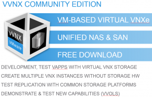
VMware now has this great new feature to be more in control of where its data blocks actually land on the storage system: VVOLs. But up until now EMC didn’t have a system capable of actually providing the back end for that. Until now I said. Starting with the VNXe 3200 all storage arrays are made VVOL capable and you can play around with that yourself. FOR FREE! The Software Defined VNX is now a reality!The good part is that this VNX to play around with is free and community supported.
This virtual VNX is actually a VM based virtual VNXe 3200.
Is it supported in production environments? NO. But it’s a VM and there’s plenty of people who you can reach out to who are willing to share their knowledge on VNXe and the VVOL technology (I hope). The first place I’d look is ECN itself. This forum is a great way to get your questions out to the experts and lots of them are actually EMC people!!
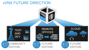
And it looks like EMC means business with this virtual machine. There is already some sort of roadmap available, so what’s keeping you from trying?
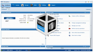
It looks like the actual Unisphere you’ll get when you are running a physical VNXe 3200, so that means it’s intuitive and therefore easy to use. Why don’t you try the VVOL feature? I know that VMware community is waiting to try it out!! VNXe 3200 AFAAnother great new feature of the entry level VNXe 3200 is tha AFA model. AFA stands for All Flash Array and for what EMC says it’s very affordable and available with 3 TiB of FLASH and up for as little as the cost of a small car. Well, in the Netherlands anyway, I know cars are a bad analogy, since the NL is probably the last place you want to buy a car. Anyway. It’s supposed to be able to deliver a stunning 75 k IOps in this 3 TiB configuration and it can go even higher if you expand the machine with more drives. It’s actually tested in a 1:1 R/W environment with 8 KiB blocks. SummaryFor me and my fellow VMware colleagues, the Software Defined VNX is probably the best thing so far, since twe can now finally test and play with this new VVOL thing and it’s free as well! Enjoy your downloads! |
20 Jun 07:04

Gone but Not Forgotten
by Allen Ward
My mini series on VMAX3 has taken a rest as I prepared for EMC World here in Vegas. I'm writing this from the EMC Elect Lounge deep in the heart of the EMC Social Lounge. I just want to take a few minutes to assure you that I'm gaining lots of insight
|
20 Jun 07:02

EMC is giving away ScaleIO as in FREE
by Keith Townsend
EMC is giving away ScaleIO for free. ScaleIO is EMC’s Server SAN product. It’s a rapidly growing category. Wikibon’s Stu Miniman just led a session at Interop (slides here) talking about the impact of Server SANs growth on traditional storage
|
20 Jun 07:01

[labbuildr]new SQL Installers available soon in beta4
by Karsten Bott
i am currently working on new SQL installers and SCVMM installers, that will also download the Required SCVMM and SQL Binaries. From Monday, 11th of May, the new Installers will be online. The attached DB is a download dummy for the AAG Scenario and will be automatically loaded as well |
20 Jun 07:01

Configuring XtremIO & RecoverPoint for VMware SRM
by Itzik Reich
One of the software that VMware have released back in 2008 and that was always my favorite after vSphere itself was always SRM (Site Recovery Manager), back then, I installed it in so many customer sites and even have a session about it at VMworld 2009 as one of the first production installation at a customer site..back then configuring the SRA (the “communicator / translator” between the vCenter to the storage array) was a pretty difficult task and im so glad things have changes so drastically over the years, im also very happy to see that as of SRM 5.8 (and of course 6.0), it has been fully merged into the vCenter web interface as seen below
another new feature is that there is No need to manage IP address changes on an individual level anymore (though those options do remain if needed). These can now be mapped from one subnet to another and applied at the Site>Network Mapping level. There is the option of using both, eg. Subnet mapping for the subnet, and individual mapping for VMs within that subnet
also, as part of VMware global initiative to not force you the customer you use MS-SQL or ORacle DB, you can now use the embedded vPostgres Database option that is built into the installer for SRM. It is an additional option beyond the currently available Databases and is supported, though not tested, up to the SRM maximums. There isn’t a way to convert or migrate an existing database to vPostgres.
SRM Architecture •Site Recovery Manager is designed for virtual-to-virtual recovery for the VMware vSphere environment •Built for two-site scenario, but can protect bi-directionally. Can also protect multiple production sites and recover them into a single, “shared recovery site”. •Site Recovery Manager integrates with third-party storage-based replication (also known as array-based replication) to move data to the remote site, our focus in this post is the RecoverPoint / XtremIO SRA Script: Site Recovery Manager is designed for the scenario that we see our customers most commonly implementing for disaster recovery—two datacenters. Site Recovery Manager supports both bi-directional failover as well as failover in a single direction. In addition, there is also support for a “shared recovery site”, allowing customers to failover multiple protected sites into a single, shared recovery site. The key elements that make up a Site Recovery Manager deployment: -VMware vSphere: Site Recovery Manager is designed for virtual-to-virtual disaster recovery. It works with many versions of ESX and ESXi (consult product documentation for more details). Site Recovery Manager also requires that you have a vCenter Server management server at each site; these two vCenter Servers are independent, each managing its own site, but Site Recovery Manager makes them aware of the virtual machines that they will need to recover if a disaster occurs. -Site Recovery Manager service: the Site Recovery Manager service is the disaster recovery brain of the deployment and takes care of managing, updating, and executing disaster recovery plans. Site Recovery Manager ties in very tightly with vCenter Server — in fact, Site Recovery Manager is managed via a vCenter Server plug-in. -Storage: Site Recovery Manager requires iSCSI, FibreChannel, or NFS storage that supports replication at the block level. in our case, we support FC /iSCSI -Storage-based (also called array-based) replication: Site Recovery Manager relies on storage vendors’ array-based replication to get the important data from the protected site to the recovery site. Site Recovery Manager communicates with the replication via storage replication adapters that the storage vendor creates and certifies for Site Recovery Manager. VMware is working with a broad range of storage partners to ensure that support for Site Recovery Manager will be available regardless of what storage a customer chooses, so expect the list to continue to grow. -vSphere Replication has no such restrictions on use of storage-type or adapters.
User Interface
Users can manage both protected and recovery SRM instances from a single UI interface, obviating the need to open multiple clients or run particular management tasks from a specific location. This is completely independent of vCenter Linked Mode. Linked mode is still helpful, because it will automatically migrate SRM licenses from site to site as VMs are migrated or fail, and also for standard non-SRM related infrastructure management. SRM 5.8 /6.0 is fully supported with the vSphere Web Client and no longer available for use with the vSphere Client. in the case of RecoverPoint / XtremIO there is a special UI to cover two very specific features SRM itself can only failover to the last point in time which isnt that helpful, especially in our case, you see, the value of RecoverPoint/ XtremIO is the ability to go to ANY point in time, so we can leverage the vCenter plugin to select the point in time you want to failover to and then SRM “think” it’s the last point in time (see a screenshot below)
the other special feature is the ability to give you, the vSphere admin or the storage admin tge insight to see which VMs are protected, which VMs aren’t and which VMs are partially protected, this is done with the unique integration of the RecoverPoint GUI to vCenter (as seen below)
Array Replication
If using storage-based replication, integration with the arrays with vendor-specific replication and protection engines are a very fundamental. This integration is provided via code written by the array vendors themselves. the SRA for RecoverPoint that support XtremIO is 2.0.2 SRAs have advanced for SRM 5, improving the integration with array-replication software for functionality like reprotect/replication reversal and failback.
SRA information is enhanced within SRM 5 and shows not only information about paired remote devices, datastores, and relevant protection groups, but will also show an arrow indicating the direction of replication for each device. This gives very quick visibility into what is being protected and to where. This is particularly important during reprotect and failback operations. Installing & Configuring the XtremIO / RecoverPoint SRA The installation itself is pretty trivial, just download the SRA form the VMware SRM web site and install the executable at both the SRM servers or in my lab case, the vCenter servers which are also acting as the SRM servers, once the SRA have been installed, you will have to restart the SRM service.
once everything is installed, you will have to configure the SRA using the SRM web interface, configuring it gets as simple as it can gets, basically, you need to point the SRA to the RecoverPoint virtual management IP and feed it with the username / password to manage the RPA’s cluster, you will need to then repeat it at the recovery site as well.
lastly, in order for the SRM SRA to control RecoverPoint, you need to change the management of the consistency group (CG) to SRM, again, this will allow RecoverPoint to be managed by an “external application” which is in our case, VMware SRM Storage Layout
lets take a look at the example above, at the protected site I have couple of datastores, each one can contain 1 VM or more, each datastore (lun at the storage level) can be a part of a protection group however, if you take a look at the purple example, a vm CAN spab across multiple datastores and hence, the protected group can span across multiple datastores (luns) then, on the right side (my recovery side),I define the recovery group which is really a logical container for the protected groups I put inside of it.
By ensuring virtual machines are stored in a logical fashion on disk according to their protection group, administrators can minimize “shuffling” of VMs to fit optimal layouts for SRM. VMDKs of a similar priority, or that will belong to the same protection group should be stored in the same datastores to minimize the amount of replication required to create efficient protection groups and thereby recovery plans. Ensuring that your storage layout and VM placement has been organized with this in mind will mitigate many issues. Workflows and Use Cases Planned Migration Allows for a data synchronization as part of the process, Will stop on errors and allow you to resolve them before continuing Since it shut’s down the virtual machines being migrated, application consistent VM’s are recovered on the recovery side! DR Event Allows for a data synchronization as part of the process, Will not stop on errors If the protected site is available, than the virtual machines being migrated will be application consistent at the recovery side. If the protected site is not available the consistency state will be what was designed in the solution. Test Recovery Allows for a data synchronization as part of the process, Supports a recovery that uses a different network, uses a clone or snapshot for the test. Reprotect Can be run following a successful recovery. Reverses the direction of replication, and protects virtual machines back to the original site. This enables a failback to recover the environment back to the primary site. Cleanup This is done following a test recovery. Removes the snapshot or clone created during the test. Powers off and deletes test VMs. Recreates the shadow VM indicating protection of the relevant VM from the primary site. The cleanup creates its own history report. Following a cleanup, the relevant plan is once again ready to be run. Use Cases Unplanned Failover Recover from unexpected site failure, Full or partial site failure. The most critical but least frequent use-case. Unexpected site failures do not happen often. When they do, fast recovery is critical to the business Preventive Failover Anticipate potential datacenter outages, For example: in case of planned hurricane, floods, forced evacuation, etc.Initiate preventive failover for smooth migration. Graceful shutdown of VMs at protected site. leverage SRM ‘planned migration’ capability to ensure no data-loss Planned Migration Most frequent SRM use case, Planned datacenter maintenance, Global load balancing. Ensure smooth site migrations. Test to minimize risk. Execute partial failovers Use SRM planned migration to minimize data-loss. Automated Failback enables bi-directional migrations Running a Test Recovery Plan
SRM offers two UI buttons to run test recoveries, or a test may alternately be initiated through a call to the API. Note the “Synchronize storage” option. This ensures very current copies of the VMs for the test.
This is a test recovery ready for users to test. Cleanup would occur after testing is complete by simply pressing the “cleanup” button. The virtual machines run from the cloned / snapshot environment at the recovery site, and replication and protection of the protected environment is not impacted during tests. Following a cleanup, there is are no running virtual machines associated with the recovery plan that was tested, and associated snapshots / clones created by the test plan have been eliminated. Shadow VMs have been recreated on the recovery site to indicate those VMs that are protected on the primary site and will be instantiated on the recovery site when a recovery plan is run. Running a Recovery Plan
Two different UI buttons can start recoveries, or alternately it may be executed by an API call. A recovery plan can be run as either a Planned Migration, or a DR event. Note that both types of execution will attempt to synchronize storage early in the recovery. The data synchronization attempt is to ensure application consistency, and will execute as an early initial step in a recovery plan after an attempt to shut down the protected VMs, to ensure data is recent and synchronized after the VMs are quiescent. Planned Migration
The difference between a Planned Migration and a Disaster Recovery is that a Planned Migration will automatically stop on errors and allow the administrator to fix the problem. A Planned Migration is designed to ensure maximum consistency of data and availability of the environment. A DR scenario is instead designed to return the environment to operation as rapidly as possible, regardless of errors. Disaster Recovery
If a Recovery Plan is run as a disaster recovery, the goal is an aggressive Recovery Time Objective, and SRM will not halt the plan from continuing regardless of any errors that might be encountered. Running a Recovery Plan – Storage Layer
Notice that during a recovery plan execution, replication is interrupted. The mirror image, or replication destination datastore, is now promoted and made read/write. The virtual machines in it are registered in vCenter in place of the shadow VM placeholders. Failback is a process of “Reverse Recovery”
Failback combines recovery plans and reprotect. “Failback” is the capability of running a recovery plan *after* an environment has been migrated or failed-over to a recovery site, to return the environment back to its starting site. After a failover has occurred, the environment can be reprotected back to the original environment once it is again safe. Following this reprotect the recovery plan can be run once more, moving the environment back to its initial primary site. Next it is imperative to reprotect once more, to ensure the environment is once again protected and ready to failover. With SRM 5 VMware introduced the “Reprotect” and failback workflows that allowed storage replication to be automatically reversed, protection of VMs to be automatically configured from the “failed over” site back to the “primary site” and thereby allowing a failover to be run that moved the environment back to the original site. After running a *planned failover only*, the SRM user can now reprotect back to the primary environment: Planned failover shuts down production VMs at the protected site cleanly, and disables their use via GUI. This ensures the VM is a static object and not powered on or running, which is why we have the requirement for planned migration to fully automate the process. Once the reprotect is complete a failback is simply the process of running the recovery plan that was used to failover initially. ok, if you have read to this point, you probably want to see it all in action, please see a demo I made showing the integration of VMware SRM and XtremIO/RecoverPoint  |


31 May 20:10

Top reasons why enterprises should choose Azure SQL Data Warehouse
by SQL Server Team
Guest post by Tiffany Wissner, Senior Director, Data Platform
Yesterday at Microsoft’s Ignite conference, we demoed the first sneak peek of Azure SQL Data Warehouse. As you build more applications in the cloud and with the increase in cloud-born data, there is strong customer demand for a data warehouse solution in the cloud to manage large volumes of structured data and to process this data with relational processing for fast analytics. Customers also want to take advantage of the cost-efficiencies, elasticity and hyper-scale of cloud for their large data warehouses. They need for that data warehouse to work with their existing data tools, utilize their existing skills and integrate with their many sources of data.
To help address this need, last week at Build, we announced an enterprise-class elastic data warehouse in the cloud called Azure SQL Data Warehouse. There’s a number of distinctive features we’d like to highlight -- including the ability to dynamically grow and shrink compute in seconds independent of storage, enabling you to pay only for the query performance you need. In addition customers can choose to simply pause compute so that you only incur compute costs when needed. The Azure SQL Data Warehouse service gives customers the ability to combine relational and non-relational data hosted in Hadoop using PolyBase.
Azure SQL Data Warehouse is a combination of enterprise-grade SQL Server augmented with the massively parallel processing architecture of the Analytics Platform System, which allows the SQL Data Warehouse service to scale across very large datasets. It integrates with existing Azure data tools including Power BI for data visualization, Azure Machine Learning for advanced analytics, Azure Data Factory for data orchestration and movement as well as Azure HDInsight, our 100% Apache Hadoop service for big data processing.

Here are five reasons why enterprises should choose Azure SQL Data Warehouse:
1) Enterprise-class cloud data warehouse built on SQL Server
SQL Data Warehouse extends the SQL Server family of products by extending the massive scale Analytics Platform System into the cloud. By offering an enterprise-class cloud data warehouse based on SQL Server, customers can take advantage of the developer skills and knowledge built over years working with the most widely deployed database in the world. The SQL Data Warehouse extends the T-SQL constructs you’re already familiar with to create indexes, partitions and stored procedures, which allows you to easily migrate to the cloud. With native integrations to Azure Data Factory, Azure Machine Learning and Power BI, customers are able to quickly ingest data, utilize learning algorithms, and visualize data born either in the cloud or on-premises. Watch the Build announcement video below for an overview of Azure SQL Data Warehouse and the integration of other Azure data services to help you gain insight into your business.
2) Separating compute and storage enables a data warehouse to meet your needs
Azure SQL Data Warehouse independently scales compute and storage so customers only pay for the query performance they need. Unlike other cloud data warehouses that require hours or days to resize for additional compute power, SQL Data Warehouse allows customers to grow or shrink query compute in seconds. Since compute and storage scale independently, costs are much easier to forecast when compared to other competitive offerings. SQL Data Warehouse offers the right balance of compute and storage to meet your needs when you need them. This means that as a customer you can scale your resources based as your needs grow rather than invest in infrastructure for the future.

3) Pause an instance to save costs
Dynamic pause enables customers to optimize the utilization of the compute infrastructure by ramping down compute while persisting the data. With other cloud vendors, customers are required to back up the data, delete the existing cluster, and, upon resume, generate a new cluster and restore data. This is both time consuming and complex for scenarios such as data marts or departmental data warehouses that need variable compute power.
4) PolyBase in the cloud makes combining data sets easy
With the incredible growth of all types of data, the need to combine structured and unstructured data is essential. With PolyBase, SQL Data Warehouse offers the ability to combine data sets easily. SQL Data Warehouse can query unstructured and semi-structured data stored in Azure Storage, Hortonworks Data Platform, or Cloudera using familiar T-SQL skills making it easy to combine data sets no matter where it is stored. Other vendors, follows the traditional data warehouse model that requires data to be moved into the instance to be accessible. SQL Data Warehouse allows the data to stay in Hadoop and combine the results with relational data via common T-SQL constructs. This keeps your data costs low and lets you choose the query speed that you need.
5) Hybrid infrastructure supports your needs on-premises and/or in the cloud
The SQL Data Warehouse service is an extension of the SQL Server family of products that offers an additional choice of data management to suit your business needs. Through support for a variety of first- and third-party products, the SQL Data Warehouse enables you to use the tools you use today to access, manage, manipulate and visualize data for faster insights. With SQL Data Warehouse you are able to quickly move to the cloud without having to move all of your infrastructure along with it. With the Analytics Platform System, Microsoft Azure and Azure SQL Data Warehouse, you can have the data warehouse solution you need on-premises, in the cloud or a hybrid solution.
To learn more about Azure SQL Data Warehouse, click here. You can also sign-up here to be notified once Azure SQL Data Warehouse preview is available later this year.
31 May 20:10
Risk When Using Dynamic Memory within Hyper-V
by Tim Radney
Virtualization is very popular for organizations: it allows them to better utilize hardware by combining multiple servers onto a single host, provides HA capabilities, and gives a reduction in various costs like heating/cooling, SQL Server licenses, and hardware. I’ve been involved in numerous projects with organizations to help them migrate from physical to virtual environments and have helped them experience these benefits.
What I want to share with you in this article is a peculiar issue I came across while working with Hyper-V on Windows Server 2012 R2 using Dynamic Memory. I must admit that most of my knowledge of virtualization has been with VMware, however that’s changing now.
When working with SQL Server on VMware I always recommend to set reservations for memory so when I encountered this Dynamic Memory feature with Hyper-V I had to do some research. I found an article (Hyper-V Dynamic Memory Configuration Guide) that explains many of the benefits and system requirements for using Dynamic Memory. This feature is pretty cool in how you can provide a virtual machine with more or less memory without it having to be powered off.
Playing around with Hyper-V I’ve found provisioning virtual machines to be straightforward and easy to learn. With little effort I was able to build a lab environment to simulate the experience my customer was having. Credit goes to my boss for providing me with awesome hardware to work with. I am running a Dell M6800 with an i7 processor, 32GB of RAM and two 1TB SSDs. This beast is better than a lot of servers I have worked on.
Using VMware Workstation 11 on my laptop, I created a Windows Server 2012 R2 guest with 4 vCPUs, 24GB of RAM and 100GB of storage. Once the guest was created and patched I added the Hyper-V role and provisioned a guest under Hyper-V. The new guest was built with Windows Server 2012 R2 with 2 vCPUs, 22GB of RAM and 60GB of storage running SQL Server 2014 RTM.
I ran three sets of tests, each using dynamic memory. For each test I used Red Gate's SQL Data Generator against the AdventureWorks2014 database to fill up the buffer pool. For the first test I started with 512MB for the Startup RAM value since that is the minimum amount of memory to start Windows Server 2012 R2 and the buffer pool stopped increasing at around 8GB.

For each test I would truncate my test table, shut down the guest, modify the memory settings and start the guest back up. For the second test I increased the Startup RAM to 768MB and the buffer pool only increased to just over 12GB in size.

For the third and final test increased the Startup RAM to 1024MB, ran the data generator and the buffer pool was able to increase to just under 16GB.

Doing a little math on these values shows that the buffer pool can’t grow more than 16 times the Startup RAM. This can be very problematic for SQL Server if the Startup RAM is less than 1/16 the size of the maximum memory. Let’s think about a Hyper-V guest with 64GB of RAM running SQL Server with a Startup RAM value of 1GB. We’ve observed that the buffer pool would not be able to use more than 16GB with this configuration, but if we set the Startup RAM value to 4096MB then the buffer pool would be able to increase 16 times allowing us to use all 64GB.
The only references I could find about why the buffer pool is limited to 16 times the Startup RAM value were on pages 8 and 16 in the whitepaper, Best Practices for Running SQL Server with HVDM. This document explains that since the buffer cache value is computed at startup time, it is a static value and doesn’t grow. However if SQL Server detects that Hot Add Memory is supported then it increases the size reserved for the virtual address space for the buffer pool by 16 times the startup memory. This document also states that this behavior affects SQL Server 2008 R2 and earlier, however my test were conducted on Windows Server 2012 R2 with SQL Server 2014 so I will be contacting Microsoft to get the best practices document updated.
Since most production DBAs do not provision virtual machines or work heavily in that space, and virtualization engineers are not studying the latest and greatest SQL Server technology, I can understand how this important information about how the buffer pool handles Dynamic Memory is unknown to a lot of people.
Even following the articles can be misleading. In the article Hyper-V Dynamic Memory Configuration Guide, the description for Startup RAM reads:
Specifies the amount of memory required to start the virtual machine. The value needs to be high enough to allow the guest operating system to start, but should be as low as possible to allow for optimal memory utilization and potentially high consolidation ratios.
Optimal memory utilization for whom, the host or the guest? If a virtualization admin was reading this, they would likely determine that it means the minimum memory allowed to start the operating system.
Being responsible for SQL Server means we need to know about other technologies that can influence our environment. With the introduction of SANs and virtualization we need to fully understand how things in those environments can negatively impact SQL Server and, more importantly, how to effectively communicate concerns to the people responsible for those systems. A DBA doesn’t necessarily need to know how to provision storage in a SAN or how to provision or be able to administer a VMWare or Hyper-V environment, but they should know the basics of how things work.
By knowing basics about how a SAN works with storage arrays, storage networks, multi-pathing and so on, as well as how the hypervisor works with the scheduling of CPUs and storage allocation within virtualization, a DBA can better communicate and troubleshoot when issues arise. Over the years I have successfully worked with a number of SAN and virtualization admins to build standards for SQL Server. These standards are unique to SQL Server and don’t necessarily apply to web or application servers.
DBAs can’t really rely on SAN and virtualization admins to fully understand best practices for SQL Server, regardless of how nice that would be, so we need to educate ourselves the best we can on how their areas of expertise can impact us.
During my testing I used a query from Paul Randal's blog post, Performance issues from wasted buffer pool memory, to determine how much buffer pool the AdventureWorks2014 database was using. I have included the code below:
SELECT
    (CASE WHEN ([database_id] = 32767)
        THEN N'Resource Database'
        ELSE DB_NAME ([database_id]) END) AS [DatabaseName],
    COUNT (*) * 8 / 1024 AS [MBUsed],
    SUM (CAST ([free_space_in_bytes] AS BIGINT)) / (1024 * 1024) AS [MBEmpty]
FROM sys.dm_os_buffer_descriptors
GROUP BY [database_id];
This code is also great for troubleshooting which of your databases is consuming the majority of your buffer pool so you can know which database you should focus on tuning the high-cost queries. If you are a Hyper-V shop, check with your admin to see if Dynamic Memory could be configured in such a way that it is negatively impacting your server.
The post Risk When Using Dynamic Memory within Hyper-V appeared first on SQLPerformance.com.
31 May 20:09


Azure SQL Data Warehouse
by James Serra
Analytics Platform System (APS) is Microsoft’s massively parallel processing (MPP) data warehouse technology. This has only been available as an on-prem solution (see video Overview of Microsoft Analytics Platform System). Until now. At the recent Microsoft Build Developer Conference, Executive Vice President Scott Guthrie announced the Azure SQL Data Warehouse (SQL DW). This is a cloud data warehouse-as-a-service (DWaaS) that will compete with Amazon’s Redshift.
But it has some additional benefits over Redshift:
- With Redshift you must scale your data warehouse by increasing both the compute and storage units. With SQL DW, compute and storage is decoupled so you can scale them individually. This is a very different economic model that can save customers a lot of money as you don’t have to purchase additional storage when you just need more compute power, or vice-versa
- The ability to pause compute when not in use so you only pay for storage, as opposed to Redshift in which you are billed 24/7 for all the VM’s that make up the nodes in your cluster
- With Redshift you have to pick a pre-defined size and it can take hours to days to resize. With SQL DW you can start small and grow or shrink in seconds
- And keep in mind with Microsoft you can have a hybrid architecture that can use an on-prem APS combined with a SQL DW, allowing you to keep sensitive data on-prem and non-sensitive data in the cloud if you wish. With Redshift you only have the option of keeping all your data in the cloud
- There is also a lot more compatibility with SQL DW as it supports many features that Redshift does not, such as indexes, stored procs, SQL UDFs, partitioning, and constraints
SQL DW is built with the same technology as APS, except that instead of using SQL Server 2014 it uses version 12 of Azure SQL Database. It also includes PolyBase. PolyBase allows APS and SQL DW to query data in a Hadoop cluster, either directly or by pushing some of the work to Hadoop itself so the query is actually run using the Hadoop clusters CPU’s. The Hadoop data is made to look as if it were local to the data warehouse, so that end-users can use their existing skill sets to query it via SQL or any reporting tool that using SQL (like Excel, SSRS, Power BI, etc). PolyBase can integrate with Hadoop in this manner via a Microsoft HDInsight cluster that can either be inside APS or in the cloud, or via a Hortonworks or Cloudera cluster.

SQL DW will work with existing data tools including Power BI for data visualization, Azure Machine Learning for advanced analytics, Azure Data Factory for data orchestration and Azure HDInsight.
The preview for Azure SQL Data Warehouse will be available later this calendar year. You can sign up to be notified when the Azure SQL Data Warehouse preview becomes available.
I will have a lot more blogs about this new service in the coming months, so stay tuned!
More info:
Microsoft BUILDs its cloud Big Data story
Microsoft Announces Azure SQL Database elastic database, Azure SQL Data Warehouse, Azure Data Lake
Introducing Azure SQL Data Warehouse
Short introduction video SQL Data Warehouse – YouTube
Top reasons why enterprises should choose Azure SQL Data Warehouse
Video on new SQL Server 2016 features and SQL DW (minute 59 with demo): The SQL Server Evolution
Video Microsoft Azure SQL Data Warehouse Overview
Video Azure SQL Data Warehouse: Deep Dive
31 May 20:09

Inconsistent analysis in read committed using locking
Well, I had a second post already planned and partially written but a comment on the first post (in what’s going to become a multi-part series) has made me decide to do a different part 2 post. So, make sure you read this post first: Locking, isolation, and read consistency.
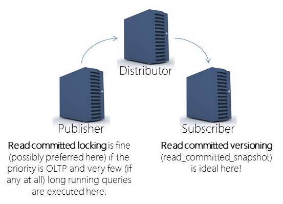
The comment was about how read committed using locking has inconsistencies – and, yes, that’s true. Read committed using locking is prone to multiple inconsistencies; there are things you can do to reduce some anomalies but in a highly volatile OLTP environment you will get inconsistencies for long running readers. This is why having a secondary server for analysis is always a great idea. Then, everyone gets the same version of the truth – the point in time to which the secondary was updated (is that nightly, weekly, monthly?). Now, if the secondary is getting updates through transactional replication, you are back to the same problem. But, here, I cannot imagine NOT using read committed with versioning. Probably one of the BEST places to use versioning is on a replication subscriber. Replication won’t be blocked by readers and readers won’t be blocked by replication:
Why is read committed with versioning preferred for readers?
More and more, we’re being tasked with analyzing “current” data. This is harder and harder to do without introducing anomalies. So, I’ll discuss non-repeatable reads in the bounds of a single statement. To get this to occur with a small data set and without setting up a bunch of connections, etc. I’ll engineer the anomaly.
Example
To do this, I’m going to use a sample database called Credit. You can download a copy of it from here. Restore the 2008 database if you’re working with 2008, 2008R2, 2012, or 2014. Only restore the 2000 database if you’re working with 2000 or 2005 (but, you can’t do versioning on 2000 so this is a 2005 or higher example).
Also, if you’re working with SQL Server 2014, you’ll potentially want to change your compatibility mode to allow for the new cardinality estimation model. However, I often recommend staying with the old CE until you’ve done some testing. To read a bit more on that, check out the section titled: Cardinality Estimator Options for SQL Server 2014 in this blog post.
So, to setup for this example – we need to:
(1) Restore the Credit sample database
(2) Leave the compatibility mode at the level restored (this will use the legacy CE). Consider testing with the new CE but for this example, the behavior (and all examples / locking, etc.) don’t actually change.
Scenario / example
(3) This is where things will get a bit more interesting – you’ll need a couple of windows to create the scenario…
FIRST WINDOW – setup the table:
USE [Credit];
GO

IF OBJECTPROPERTY(object_id('[dbo].[MembersOrdered]'), 'IsUserTable') = 1
    DROP TABLE [dbo].[MembersOrdered];
GO

-- Create a copy of the Member table to mess with!
SELECT *
INTO [dbo].[MembersOrdered]
FROM [dbo].[Member];
GO

-- Create a bad clustered index that's prone to both fragmentation and
-- record relocation. This is part of what makes this scenario more likely!
-- But, that's not the main point of discussion HERE. This is good
-- because it's also easy to visualize
CREATE CLUSTERED INDEX [MembersOrderedLastname]
ON [dbo].[MembersOrdered]
    ([lastname], [firstname], [middleinitial]);
GO

SELECT COUNT(*) FROM [dbo].[MembersOrdered];
GO
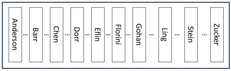
Now… we’ll engineer the problem. But, I’ll describe it visually here:
This is a rough approximation of what the data looks like when the table is clustered by lastname (not that I’m recommending that you do this).
The table has NO nonclustered indexes and ONLY a clustered index on lastname. The data is essentially ordered by lastname (not going to get technical about what the data looks like on the page here or the fact that it’s really the slot array that maintains order not the actual rows… for this example – the logical structure of the table is good enough to get the point).
(4) So, now that the table has been created – we will start by creating a problem (a row that will end up blocking us):
SECOND WINDOW – we’ll create a blocking transaction (t1)…
USE [Credit];
GO

BEGIN TRANSACTION
UPDATE [dbo].[MembersOrdered]
    SET [lastname] = 'test',
        [firstname] = 'test'
WHERE [member_no] = 9965;
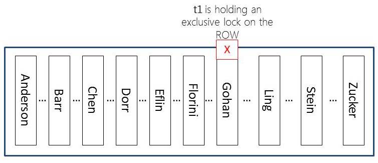
Don’t get me wrong – this is a horribly bad practice (to have interaction in the midst of a transaction and to only send part of the transaction… if you walk away – SQL Server is incredibly patient and will hold locks until the transaction is finished [or, killed by an administrator]). But, the point… now our table will essentially look like this:
Yes, there are other locks that exist but this is the only one we really care about here…
And, yes, there are MORE locks than just what I show here. SQL Server will also hold an IX lock on the page where this row resides and an IX lock on the table as well. And, of course, SQL Server will also hold a shared lock on the database. All of these locks (IX and the database-level S lock) are used as indicators. Individually, they don’t really block all that many other operations. You can have MANY IX locks on the same page at the same time and you can have many IX locks on the same table at the same time. Essentially these locks are used to show that someone has the “intent” to exclusively lock resources on this resource.
If you’re interested, check out sys.dm_tran_locks to see the locks held at each point of this example…
(5) So, now that the table has a locked row, we will try again to get a row count. Go back to the FIRST WINDOW and JUST re-run the query to get a count:
SELECT COUNT(*) FROM [dbo].[MembersOrdered];
GO
This will be blocked. And, it will sit blocked until the transaction finishes (either through a commit or rollback OR by being killed – none of which we’ll do…yet ).
So, what’s interesting and we need a bit of back-story to fill in is that our count query reads ONLY committed rows (we know that – it’s read committed locking). What a lot of people don’t know is that the row-level shared locks are released as soon as the resource has been read. This is to reduce blocking and because there’s no need (in read committed ) to preserve the state of the row (like repeatable reads does). And, I’ll prove that with an update…
(6) Now we’ll update a row that’s just sitting there and not locked (but, may have already been counted [locked, read, and then the lock was released] by our count query).
THIRD WINDOW – update and move a row that was already counted
USE [Credit];
GO

UPDATE [dbo].[MembersOrdered]
 SET [lastname] = 'ZZZuckerman',
 [firstname] = 'ZZZachary'
WHERE [lastname] = 'ANDERSON'
 AND [firstname] = 'AMTLVWQBYOEMHD';
GO
OK, now here’s another horribly bad practice (not using a key for a modification). But, this table has all sorts of problems (which is what makes it a wonder example for this). And, if I don’t go with something that’s efficiently indexed for this update then the locking would be different. I NEED to get row-level locking here. So, I have to do the update above. And, now what’s happened:
There are so many bad things going on with this poor table. What if there are two rows with that name (ok, unlikely) but you still shouldn’t do modifications without a KEY (primary / or candidate)!
(7) Now, it’s time to “complete” the transaction that was blocking our count query.
Go back to the SECOND WINDOW and complete the transaction (to be honest, you can COMMIT or ROLLBACK – it really won’t matter for this example):
ROLLBACK TRANSACTION;
(8) Step 7 will have unblocked the row count query so all you need to do is go back to the first window and check the count that’s sitting there… which will be 10001 rows in our table that only has 10000 rows. Why? Because you were NOT guaranteed repeatable reads even in the bounds of a single statement.
Re-run the count query and you’ll get 10000 again.
Why read committed with versioning solves this problem?
When you change the database to read_commmitted_snapshot you change ALL read committed statements to use version-based reads. The best part is that we’ll never WAIT for in-flight rows nor will we see rows whose transactions completed within the bounds of your statement [the longer running the statements the more that this is possible]. The incorrect count would not occur for a few reasons but I’ll create a list of the reasons here:
When the row modification (t1) is made – the row will be versioned (SQL uses “copy on write” / “point in time” = snapshot) to take the BEFORE modification VERSION of the row and put it into the version store.
When the count begins it will just quickly continue (and not be blocked by the X lock held on the ‘Gohan’ row). This is not a problem, the columns are changing but the row is not being deleted – yes, we should count that row.
If I could switch to the window and run the update fast enough, it too would not be blocked by the version-based read NOR would the moved row be visible (even if it made it there in time) by the version-based read because it’s new location (handled as an INSERT) would be NEWER than our count statement’s START time. Our count will reconcile to the point in time when the statement BEGAN. Nothing is blocked and those changes (even when committed before we get there) are NOT visible to our version-based read.
Is Summary
Yes, read committed with versioning is often MUCH preferred over read committed using locking. But, versioning does come at an expense. You do need to do monitoring and analysis of THE version store (in THE tempdb). Someday (SQL Server 2016???) maybe we’ll multiple tempdbs (that would be awesome) and ideally, we’ll have some nice capabilities for controlling / limiting version store overhead (of one database over another). But, for right now – you have to make sure that your tempdb is optimized! And, if you have an optimized tempdb and you don’t have a lot of really poorly written long-running queries, then you might find out that the overhead is less than you expected. This is absolutely something that you should be not only considering but using!
Whitepaper: Working with tempdb in SQL Server 2005
Plus, be sure to review Paul’s tempdb category for other tips / tricks, etc.
OK, so now the originally planned part 2 is now trending to be part 3. Depending on questions – I’ll get to that in the next few days!
Thanks for reading,
k
The post Inconsistent analysis in read committed using locking appeared first on Kimberly L. Tripp.
31 May 20:09
Database Design: 3-State Bits
by andyleonard
I can hear you thinking, “Andy, you’re off your old rocker. There are only two states for bit values!” And you are correct. Almost. What if I’m storing a truly binary value – a value that possesses only two possible states – but there’s the possibility of a third state to indicate that I do not know which state applies. Consider this single-column example table: [Value] High Low Don’t Know or Don’t Care The two discrete states are High and Low. The 3rd state can be labeled “unknown.” Can I represent...(read more)
31 May 20:08

Identifying queries with SOS_SCHEDULER_YIELD waits
by Paul Randal
One of the problems with the SOS_SCHEDULER_YIELD wait type is that it’s not really a wait type. When this wait type occurs, it’s because a thread exhausted its 4ms scheduling quantum and voluntarily yielded the CPU, going directly to the bottom of the Runnable Queue for the scheduler, bypassing the Waiter List. A wait has to be registered though when a thread goes off the processor, so SOS_SCHEDULER_YIELD is used.
You can read more about this wait type:
You want to investigate these waits if they’re a prevalent wait on your server, as they could be an indicator of large scans happening (of data that’s already in memory) where you’d really rather have small index seeks.
The problem is that they’re not a real wait type, so you can’t use my script to look at sys.dm_os_waiting_tasks and get the query plans of threads incurring that wait type, because these threads aren’t waiting for a resource, so don’t show up in the output of sys.dm_os_waiting_tasks!
The solution is to use the sys.dm_exec_requests DMV, as that will show the last_wait_type for all running requests. Below is a script you can use.
SELECT
	[er].[session_id],
	[es].[program_name],
	[est].text,
	[er].[database_id],
	[eqp].[query_plan],
	[er].[cpu_time]
FROM sys.dm_exec_requests [er]
INNER JOIN sys.dm_exec_sessions [es] ON
	[es].[session_id] = [er].[session_id]
OUTER APPLY sys.dm_exec_sql_text ([er].[sql_handle]) [est]
OUTER APPLY sys.dm_exec_query_plan ([er].[plan_handle]) [eqp]
WHERE
    [es].[is_user_process] = 1
	AND [er].[last_Wait_type] = N'SOS_SCHEDULER_YIELD'
ORDER BY
    [er].[session_id];
GO
That will give you the code and query plan of what’s happening, but even with that it might not be obvious which exact operator is causing that wait so you may need to resort to capturing SQL Server call stacks, as I explain in the first blog post link above.
Enjoy!
The post Identifying queries with SOS_SCHEDULER_YIELD waits appeared first on Paul S. Randal.
31 May 20:08
Internals of the Seven SQL Server Sorts – Part 2
by Paul White
The seven SQL Server sort implementation classes are:
- CQScanSortNew
- CQScanTopSortNew
- CQScanIndexSortNew
- CQScanPartitionSortNew (SQL Server 2014 only)
- CQScanInMemSortNew
- In-Memory OLTP (Hekaton) natively compiled procedure Top N Sort (SQL Server 2014 only)
- In-Memory OLTP (Hekaton) natively compiled procedure General Sort (SQL Server 2014 only)
The first four types were covered in part one of this article.
5. CQScanInMemSortNew
This sort class has a number of interesting features, some of them unique:
- As the name suggests, it always sorts entirely in memory; it will never spill to tempdb
- Sorting is always performed using quicksort qsort_s in the standard C run-time library MSVCR100
- It can perform all three logical sort types: General, Top N, and Distinct Sort
- It can be used for clustered columnstore per-partition soft sorts (see section 4 in part 1)
- The memory it uses may be cached with the plan rather than being reserved just before execution
- It can be identified as an in-memory sort in execution plans
- A maximum of 500 values can be sorted
- It is never used for index-building sorts (see section 3 in part 1)
CQScanInMemSortNew is a sort class you will not encounter often. Since it always sorts in memory using a standard library quicksort algorithm, it would not be a good choice for general database sorting tasks. In fact, this sort class is only used when all its inputs are runtime constants (including @variable references). From an execution plan perspective, that means the input to the Sort operator must be a Constant Scan operator, as the examples below demonstrate:
-- Regular Sort on system scalar functions
SELECT X.i
FROM
(
    SELECT @@TIMETICKS UNION ALL
    SELECT @@TOTAL_ERRORS UNION ALL
    SELECT @@TOTAL_READ UNION ALL
    SELECT @@TOTAL_WRITE
) AS X (i)
ORDER BY X.i;

-- Distinct Sort on constant literals
WITH X (i) AS
(
    SELECT 3 UNION ALL
    SELECT 1 UNION ALL
    SELECT 1 UNION ALL
    SELECT 2
)
SELECT DISTINCT X.i
FROM X
ORDER BY X.i;

-- Top N Sort on variables, constants, and functions
DECLARE
    @x integer = 1,
    @y integer = 2;

SELECT TOP (1)
    X.i
FROM
(
    VALUES
        (@x), (@y), (123),
        (@@CONNECTIONS)
) AS X (i)
ORDER BY X.i;
The execution plans are:

A typical call stack during sorting is shown below. Notice the call to qsort_s in the MSVCR100 library:

All three execution plans shown above are in-memory sorts using CQScanInMemSortNew with inputs small enough for the sort memory to be cached. This information is not exposed by default in execution plans, but it can be revealed using undocumented trace flag 8666. When that flag is active, additional properties appear for the Sort operator:

The cache buffer is limited to 62 rows in this example as demonstrated below:
-- Cache buffer limited to 62 rows
SELECT X.i
FROM
(
    VALUES
    (001),(002),(003),(004),(005),(006),(007),(008),(009),(010),
    (011),(012),(013),(014),(015),(016),(017),(018),(019),(020),
    (021),(022),(023),(024),(025),(026),(027),(028),(029),(030),
    (031),(032),(033),(034),(035),(036),(037),(038),(039),(040),
    (041),(042),(043),(044),(045),(046),(047),(048),(049),(050),
    (051),(052),(053),(054),(055),(056),(057),(058),(059),(060),
    (061),(062)--, (063)
) AS X (i)
ORDER BY X.i;
Uncomment the final item in that script to see the Sort cache buffer property change from 1 to 0:

When the buffer is not cached, the in-memory sort must allocate memory as it initializes and as required as it reads rows from its input. When a cached buffer can be used, this memory allocation work is avoided.

The following script can be used to demonstrate that the maximum number of items for a CQScanInMemSortNew in-memory quicksort is 500:
SELECT X.i
FROM
(
    VALUES
    (001),(002),(003),(004),(005),(006),(007),(008),(009),(010),
    (011),(012),(013),(014),(015),(016),(017),(018),(019),(020),
    (021),(022),(023),(024),(025),(026),(027),(028),(029),(030),
    (031),(032),(033),(034),(035),(036),(037),(038),(039),(040),
    (041),(042),(043),(044),(045),(046),(047),(048),(049),(050),
    (051),(052),(053),(054),(055),(056),(057),(058),(059),(060),
    (061),(062),(063),(064),(065),(066),(067),(068),(069),(070),
    (071),(072),(073),(074),(075),(076),(077),(078),(079),(080),
    (081),(082),(083),(084),(085),(086),(087),(088),(089),(090),
    (091),(092),(093),(094),(095),(096),(097),(098),(099),(100),
    (101),(102),(103),(104),(105),(106),(107),(108),(109),(110),
    (111),(112),(113),(114),(115),(116),(117),(118),(119),(120),
    (121),(122),(123),(124),(125),(126),(127),(128),(129),(130),
    (131),(132),(133),(134),(135),(136),(137),(138),(139),(140),
    (141),(142),(143),(144),(145),(146),(147),(148),(149),(150),
    (151),(152),(153),(154),(155),(156),(157),(158),(159),(160),
    (161),(162),(163),(164),(165),(166),(167),(168),(169),(170),
    (171),(172),(173),(174),(175),(176),(177),(178),(179),(180),
    (181),(182),(183),(184),(185),(186),(187),(188),(189),(190),
    (191),(192),(193),(194),(195),(196),(197),(198),(199),(200),
    (201),(202),(203),(204),(205),(206),(207),(208),(209),(210),
    (211),(212),(213),(214),(215),(216),(217),(218),(219),(220),
    (221),(222),(223),(224),(225),(226),(227),(228),(229),(230),
    (231),(232),(233),(234),(235),(236),(237),(238),(239),(240),
    (241),(242),(243),(244),(245),(246),(247),(248),(249),(250),
    (251),(252),(253),(254),(255),(256),(257),(258),(259),(260),
    (261),(262),(263),(264),(265),(266),(267),(268),(269),(270),
    (271),(272),(273),(274),(275),(276),(277),(278),(279),(280),
    (281),(282),(283),(284),(285),(286),(287),(288),(289),(290),
    (291),(292),(293),(294),(295),(296),(297),(298),(299),(300),
    (301),(302),(303),(304),(305),(306),(307),(308),(309),(310),
    (311),(312),(313),(314),(315),(316),(317),(318),(319),(320),
    (321),(322),(323),(324),(325),(326),(327),(328),(329),(330),
    (331),(332),(333),(334),(335),(336),(337),(338),(339),(340),
    (341),(342),(343),(344),(345),(346),(347),(348),(349),(350),
    (351),(352),(353),(354),(355),(356),(357),(358),(359),(360),
    (361),(362),(363),(364),(365),(366),(367),(368),(369),(370),
    (371),(372),(373),(374),(375),(376),(377),(378),(379),(380),
    (381),(382),(383),(384),(385),(386),(387),(388),(389),(390),
    (391),(392),(393),(394),(395),(396),(397),(398),(399),(400),
    (401),(402),(403),(404),(405),(406),(407),(408),(409),(410),
    (411),(412),(413),(414),(415),(416),(417),(418),(419),(420),
    (421),(422),(423),(424),(425),(426),(427),(428),(429),(430),
    (431),(432),(433),(434),(435),(436),(437),(438),(439),(440),
    (441),(442),(443),(444),(445),(446),(447),(448),(449),(450),
    (451),(452),(453),(454),(455),(456),(457),(458),(459),(460),
    (461),(462),(463),(464),(465),(466),(467),(468),(469),(470),
    (471),(472),(473),(474),(475),(476),(477),(478),(479),(480),
    (481),(482),(483),(484),(485),(486),(487),(488),(489),(490),
    (491),(492),(493),(494),(495),(496),(497),(498),(499),(500)
--,    (501)
) AS X (i)
ORDER BY X.i;
Again, uncomment the last item to see the InMemory Sort property change from 1 to 0. When this happens, CQScanInMemSortNew is replaced by either CQScanSortNew (see section 1) or CQScanTopSortNew (section 2). A non-CQScanInMemSortNew sort may still be performed in memory, of course, it just uses a different algorithm, and is allowed to spill to tempdb if necessary.
6. In-Memory OLTP natively compiled stored procedure Top N Sort
The current implementation of In-Memory OLTP (previously code-named Hekaton) natively-compiled stored procedures uses a priority queue followed by qsort_s for Top N Sorts, when the following conditions are met:
- The query contains TOP (N) with an ORDER BY clause
- The value of N is a constant literal (not a variable)
- N has a maximum value of 8192; although
- The presence of joins or aggregations may reduce the 8192 value as documented here
The following code creates a Hekaton table containing 4000 rows:
CREATE DATABASE InMemoryOLTP;
GO
-- Add memory optimized filegroup
ALTER DATABASE InMemoryOLTP
ADD FILEGROUP InMemoryOLTPFileGroup
CONTAINS MEMORY_OPTIMIZED_DATA;
GO
-- Add file (adjust path if necessary)
ALTER DATABASE InMemoryOLTP
ADD FILE
(
	NAME = N'IMOLTP',
	FILENAME = N'C:\Program Files\Microsoft SQL Server\MSSQL12.SQL2014\MSSQL\DATA\IMOLTP.hkf'
)
TO FILEGROUP InMemoryOLTPFileGroup;
GO
USE InMemoryOLTP;
GO
CREATE TABLE dbo.Test
(
    col1 integer NOT NULL,
    col2 integer NOT NULL,
    col3 integer NOT NULL,

    CONSTRAINT PK_dbo_Test
    PRIMARY KEY NONCLUSTERED HASH (col1)
    WITH (BUCKET_COUNT = 8192)
)
WITH
(
    MEMORY_OPTIMIZED = ON,
    DURABILITY = SCHEMA_ONLY
);
GO
-- Add numbers from 1-4000 using
-- Itzik Ben-Gan's number generator
WITH
  L0   AS (SELECT 1 AS c UNION ALL SELECT 1),
  L1   AS (SELECT 1 AS c FROM L0 AS A CROSS JOIN L0 AS B),
  L2   AS (SELECT 1 AS c FROM L1 AS A CROSS JOIN L1 AS B),
  L3   AS (SELECT 1 AS c FROM L2 AS A CROSS JOIN L2 AS B),
  L4   AS (SELECT 1 AS c FROM L3 AS A CROSS JOIN L3 AS B),
  L5   AS (SELECT 1 AS c FROM L4 AS A CROSS JOIN L4 AS B),
  Nums AS (SELECT ROW_NUMBER() OVER(ORDER BY (SELECT NULL)) AS n FROM L5)
INSERT dbo.Test
    (col1, col2, col3)
SELECT
    N.n,
    ABS(CHECKSUM(NEWID())),
    ABS(CHECKSUM(NEWID()))
FROM Nums AS N
WHERE N.n BETWEEN 1 AND 4000;
The next script creates a suitable Top N Sort in a natively-compiled stored procedure:
-- Natively-compiled Top N Sort stored procedure
CREATE PROCEDURE dbo.TestP
WITH EXECUTE AS OWNER, SCHEMABINDING, NATIVE_COMPILATION
AS
BEGIN ATOMIC
WITH
(
    TRANSACTION ISOLATION LEVEL = SNAPSHOT,
    LANGUAGE = N'us_english'
)
    SELECT TOP (2) T.col2
    FROM dbo.Test AS T
    ORDER BY T.col2
END;
GO
EXECUTE dbo.TestP;
The estimated execution plan is:

A call stack captured during execution shows the insert to the priority queue in progress:

After the priority queue build is complete, the next call stack shows a final pass through the standard library quicksort:

The xtp_p_* library shown in those call stacks is the natively-compiled dll for the stored procedure, with source code saved on the local SQL Server instance. The source code is automatically-generated from the stored procedure definition. For example, the C file for this native stored procedure contains the following fragment:

This is as close as we can get to having access to SQL Server source code.
7. In-Memory OLTP natively compiled stored procedure Sort
Natively-compiled procedures do not currently support Distinct Sort, but non-distinct general sorting is supported, without any restrictions on the size of the set. To demonstrate, we will first add 6,000 rows to the test table, giving a total of 10,000 rows:
WITH
  L0   AS (SELECT 1 AS c UNION ALL SELECT 1),
  L1   AS (SELECT 1 AS c FROM L0 AS A CROSS JOIN L0 AS B),
  L2   AS (SELECT 1 AS c FROM L1 AS A CROSS JOIN L1 AS B),
  L3   AS (SELECT 1 AS c FROM L2 AS A CROSS JOIN L2 AS B),
  L4   AS (SELECT 1 AS c FROM L3 AS A CROSS JOIN L3 AS B),
  L5   AS (SELECT 1 AS c FROM L4 AS A CROSS JOIN L4 AS B),
  Nums AS (SELECT ROW_NUMBER() OVER(ORDER BY (SELECT NULL)) AS n FROM L5)
INSERT dbo.Test
    (col1, col2, col3)
SELECT
    N.n,
    ABS(CHECKSUM(NEWID())),
    ABS(CHECKSUM(NEWID()))
FROM Nums AS N
WHERE N.n BETWEEN 4001 AND 10000;
Now we can drop the previous test procedure (natively-compiled procedures cannot currently be altered) and create a new one that performs an ordinary (not top-n) sort of the 10,000 rows:
DROP PROCEDURE dbo.TestP;
GO
CREATE PROCEDURE dbo.TestP
WITH EXECUTE AS OWNER, SCHEMABINDING, NATIVE_COMPILATION
AS
BEGIN ATOMIC
WITH
(
    TRANSACTION ISOLATION LEVEL = SNAPSHOT,
    LANGUAGE = N'us_english'
)
    SELECT T.col2
    FROM dbo.Test AS T
    ORDER BY T.col2
END;
GO
EXECUTE dbo.TestP;
The estimated execution plan is:

Tracing the execution of this sort shows that it starts by generating multiple small sorted runs using standard library quicksort again:

Once that process is complete, the sorted runs are merged, using a priority queue scheme:

Again, the C source code for the procedure shows some of the details:

Summary of Part 2
- CQScanInMemSortNew is always an in-memory quicksort. It is limited to 500 rows from a Constant Scan, and may cache its sort memory for small inputs. A sort can be identified as a CQScanInMemSortNew sort using execution plan properties exposed by trace flag 8666.
- Hekaton native compiled Top N Sort requires a constant literal value for N <= 8192 and sorts using a priority queue followed by a standard quicksort
- Hekaton native compiled General Sort can sort any number of rows, using standard library quicksort to generate sort runs, and a priority queue merge sort to combine runs. It does not support Distinct Sort.
The post Internals of the Seven SQL Server Sorts – Part 2 appeared first on SQLPerformance.com.
31 May 20:08
Yeah My Mama She Told Me Don’t Worry About Your JOINs
by Karen Lopez

(with apologies to Meghan Trainor)
Because you know
I’m all about the data
‘Bout the data, no trouble
I’m all about the data
‘Bout the data, no trouble
I’m all about the data
‘Bout the data, no trouble
I’m all about the data
‘Bout the data
Yeah, it’s pretty clear, I ain’t NoSQL
But I can love it, love it
Like I’m supposed to do
‘Cause I still got zoom zoom that in the database
With all the right facts in all the right places
I see the newbies are workin’ that drawing slop
We know that shit ain’t real
C’mon now, make it stop
If you got data models, just raise ’em up
‘Cause a Zachman Framework is perfect
From the bottom to the top
Yeah, my mama she told me don’t worry about your joins
She says, “Data likes a little quality to keep it right.”
You know I won’t be no schemafree denormal Barbie doll
So if that’s what you’re into then go ahead and move along
Because you know I’m
All about the data
‘Bout the data, no trouble
I’m all about the data
‘Bout the data, no trouble
I’m all about the data
‘Bout the data, no trouble
I’m all about the data
‘Bout the data
Hey!

I’m bringing quality facts
Go ahead and tell polyschematics that
Normalized data, I know you think it’s slow
But I’m here to tell ya
Transactional data’s perfect from the bottom to the top
Yeah my mama she told me don’t worry about your joins
She says, “Data likes a little quality to keep it right.”
You know I won’t be no schemafree denormal Barbie doll
If eventual consistency’s your thing then move along
Because you know I’m
All about the data
‘Bout the data, no trouble
I’m all about the data
‘Bout the data, no trouble
I’m all about the data
‘Bout the data, no trouble
I’m all about the data
‘Bout the data
Because you know I’m
All about the data
‘Bout the data, no trouble
I’m all about the data
‘Bout the data, no trouble
I’m all about the data
‘Bout the data, no trouble
I’m all about the data
‘Bout the data
Because you know I’m
All about the data
‘Bout the data, no trouble
I’m all about the data
‘Bout the data, no trouble
I’m all about the data
‘Bout the data, no trouble
I’m all about the data
‘Bout the data
‘Bout the data, ’bout the data
Hey, hey, ooh
You know you love the data

31 May 20:07
Data Stories….
by Karen Lopez
")
I prefer to think of it is trying to decipher the stories data is already saying. So more listening, less torture.
31 May 20:02
7 Databases in 70 Minutes
by Karen Lopez
Lara Rubbelke (@sqlgal ) and I recently presented 7 Databases in 70 Minutes, a sort of homage to the book 7 Databases in 7 Weeks. The event was SQLBits, a UK-based SQL Server event. We first gave this talk at the PASS Summit last year.
We don’t talk about the same databases as the book, but the concepts are the same. We cover relational, column family, graph, key value, Hadoop, and document database technologies, focusing mostly on the reasons why you would want to consider these and what a typical create and query statement might look like.
And then we end with 7 reasons why you should start exploring them.
It’s a blast talking about so many things in such a short time frame and it’s fun watching light bulbs go off as people realize these aren’t just silly open source projects, but real, enterprise class solutions for common enterprise processes.
Check out our slide deck.
Have you been looking at non-relational technologies to tell your data stories, too?
31 May 20:01
SQL Server 2016 : In-Memory OLTP Enhancements
by Aaron Bertrand
Update: November 30, 2015
The SQL Server team has published a blog post with some new functionality for In-Memory OLTP in CTP 3.1:
Update: November 17, 2015
Jos de Bruijn has posted an updated list of In-Memory OLTP changes as of CTP 3.0:
I posted earlier about the changes to Availability Groups in SQL Server 2016, which I learned about at MS Ignite largely from a session by Joey D'Antoni and Denny Cherry. Another great session was from Kevin Farlee and Sunil Agarwal on the changes in store for In-Memory OLTP (the feature formerly known as "Hekaton"). An interesting side note: the video of this session shows a demo where Kevin is running CTP2.0 (build 13.0.200) – though it is probably not the build we'll see publicly this summer.
| Feature/Limit | SQL Server 2014 | SQL Server 2016 |
|---|---|---|
| Maximum size of durable table | 256 GB | 2 TB |
| LOB (varbinary(max), [n]varchar(max)) | Not supported | Supported* |
| Transparent Data Encryption (TDE) | Not supported | Supported |
| Offline Checkpoint Threads | 1 | 1 per container |
| ALTER PROCEDURE / sp_recompile | Not supported | Supported (fully online) |
| Nested native procedure calls | Not supported | Supported |
| Natively-compiled scalar UDFs | Not supported | Supported |
| ALTER TABLE | Not supported (DROP / re-CREATE) |
Partially supported (offline – details below) |
| DML triggers | Not supported | Partially supported (AFTER, natively compiled) |
| Indexes on NULLable columns | Not supported | Supported |
| Non-BIN2 collations in index key columns | Not supported | Supported |
| Non-Latin codepages for [var]char columns | Not supported | Supported |
| Non-BIN2 comparison / sorting in native modules | Not supported | Supported |
| Foreign Keys | Not supported | Supported |
| Check/Unique Constraints | Not supported | Supported |
| Parallelism | Not supported | Supported |
| OUTER JOIN, OR, NOT, UNION [ALL], DISTINCT, EXISTS, IN | Not supported | Supported |
| Multiple Active Result Sets (MARS) (Means better Entity Framework support.) |
Not supported | Supported |
| SSMS Table Designer | Not supported | Supported |
* LOB support will not be available in the CTP shipping this summer.
ALTER TABLE is an offline operation, and will support adding/dropping columns, indexes, and constraints. There will be new syntax extensions to support some of these actions. You can change your bucket count values with a simple rebuild (however note that any rebuild will require 2X memory):
ALTER TABLE dbo.InMemoryTable
  ALTER INDEX IX_NC_Hash
  REBUILD WITH (BUCKET_COUNT = 1048576);
In addition to these capacity / feature enhancements, there are also some additional performance enhancements. For example, there will be the ability to add an in-memory, updateable, non-clustered columnstore index over either disk-based or in-memory tables. And they have simplified the way that deleted rows are processed (in 2014, those operations use FileStream; in 2016, they will skip this step). There have also been improvements to the migration advisors and the best practices analyzer – they are now lighter on data gathering and provide more context about migration complexity.
There are still some limitations with some of these changes. TDE, as an example, requires additional steps when upgrading a database. But it's clear that as In-Memory OLTP gets more mature, they are chipping away at many of the biggest roadblocks to adoption.
But wait, there's more! If you want to use In-Memory OLTP in Azure SQL Database, there will be a public preview with full support coming this summer. So you won't need your own physical server with 2 TB of memory to push this feature to its limits. Do not expect any trickling of this feature into Standard Edition, however.
The post SQL Server 2016 : In-Memory OLTP Enhancements appeared first on SQLPerformance.com.
31 May 20:01

Monitoring skew in PDW
by Rob Farley
When you have data stored across several servers, skew becomes very significant.
In SQL Server Parallel Data Warehouse (PDW), part of the Analytics Platform System (APS), data is stored in one of two ways – distributed or replicated. Replicated data is copied in full across every compute node (those servers which actually store user data), while distributed data is spread as evenly as possible across all the compute nodes, with the decision about where each row of data is stored is dependent on the hash of a column’s value. This column is known as the distribution key.
For performance reasons, though, data warehouse designers will typically choose a distribution key that avoids data movement, by choosing a column which is typically used in joins or aggregations. This performance is traded off against skew, which itself can have a performance impact. If a disproportionate amount of data is stored on a single compute node (which is really a question of ‘distributions’ which correspond to filegroups – eight per compute node), then storage is effectively used up more quickly (after all, you only need one disk to fill up to have problems), and queries run slower because one distribution has to churn through more data than the others.
And so skew should be monitored.  This fits in nicely with this month’s T-SQL Tuesday, on the topic of monitoring, and hosted by Cathrine Wilhemsen (@cathrinew).
It’s not even just monitoring it that is important, but trending it. You see, your data can change over time.
Imagine you sell products, to customers, in stores, over time. You could distribute your data by store, product, customer, or day (or even by some surrogate key, but then you need to generate that surrogate key). And whatever you choose might start off as just fine – until your business changes a little... such as a product comes out that outsells the others by a long way, or when you start selling online, to anonymous users, and offer sales on certain days of the year. Skew might not be there at the start, but it might become a factor over time.
So how can you measure skew? Well, using DBCC PDW_SHOWSPACEUSED.
You might have created a table called dbo.Sales, but if you have six compute nodes, then your data is actually stored across 48 tables. DBCC PDW_SHOWSPACEUSED("dbo.Sales") will provide the number of rows, and the space used and reserved for each of these 48 tables, letting me see what the skew is like.
If I have 480 million rows, then ideally I have 10 million rows in each distribution. But if my data shows that 4 of my distributions have 15 million rows, and the other 44 have about 9.5 million, then it might not seem like much skew – most of them are 95% of what I had hoped for. But if the disks storing those 15 million-row tables are starting to fill up, then I’m essentially missing out on the opportunity to store 5.5 million rows on each of the 44 emptier ones – 240 million rows’ worth! To put it another way – if they were all as full as my fullest distribution, I could’ve had 48 * 15 million rows, which is 720 million rows! This is not efficient use of my storage.
Applying a bit of maths like this can help me work out the wastage – looking to see what the maximum number of rows (or storage allocated) is, and multiplying that by the number of distributions that I have, to see what I could be storing if I didn’t have skew. This wastage could be a stored as a percentage easily enough, and this can be tracked over time.
You could very easily run this command across your distributed tables on a regular basis, storing the results in a table, and produce a report which shows both the overall skew across the appliance and individually across each table. This can then become part of your capacity planning process, as I’m sure you’re considering across all your SQL Server instances.
23 May 00:45

Getting Started with Microsoft Azure
by MVP Award Program
Editor’s note: The following post was written by .Net MVP Dirk Strauss
What is Microsoft Azure?
It sometimes surprises me how little some developers know about Microsoft Azure. I would also assume that this has a lot to do with the fact that many developers get to know Microsoft Azure if and when they need to use it as part of a project they’re working on. Let’s face it, many developers abide by the architecture of the application as specified by the system architect or business analyst. So many devs need to learn Azure on their own time.
This is why I wanted to write a few articles on Microsoft Azure. For this reason, the best place to start is right at the beginning. To get the official word on exactly what Microsoft Azure is, head on over to the Azure website (http://azure.microsoft.com/en-us/overview/what-is-azure/). This is the definition of Microsoft Azure:
“In short, it’s Microsoft’s cloud platform: a growing collection of integrated services—compute, storage, data, networking, and app—that help you move faster, do more, and save money. But that’s just scratching the surface.”
Obviously the Microsoft Azure website is a great place to start, but I wanted to take you a little further. For this let’s have a look at the Azure Dashboard. What does Azure mean to me as a software developer?
Microsoft Azure Dashboard
The dashboard is very easy on the eye and the main functionality of each item is neatly listed down the left side of the page in a tabbed menu. There is so much that Azure offers, that this article will become too long if I had to write something about everything. Therefore I will focus on only a few of the items available.

Azure Web Apps
Here you can create web applications and host them on Azure. The first time you access this tab, you will be prompted to create a web app.

When you click on the Create a web app link, you will see this wizard pop up. Enter a unique name for the URL. The rest of the settings are self-explanatory.

After you have created your web app, you can navigate to the URL you specified earlier. You will see the following message:

You can view the documentation on deploying a web app in Azure at the following link: http://azure.microsoft.com/en-us/documentation/articles/web-sites-deploy/
The newly created web app will then also be listed under the web apps tab.
If you click on the arrow next to your web app name, you are able to manage the web app.

For the purposes of this article, I’ll create a web page in Visual Studio and publish that to our web app on Azure.

The web application I created in Visual Studio is nothing complex. It’s just a demo page to illustrate the power of Azure and publishing from Visual Studio. You can create any web app you wish, for example testing some or other functionality you want to use or playing around with a new SDK.

When you are ready to publish, right click on the project and click on the ‘Publish Web Site’ link from the context menu.

You will notice that Microsoft Azure Websites is listed as a publish target.

When I click on this, because I’m already logged in to Azure, Visual Studio shows me that I’m signed in and lists all my existing websites. I can now select the web site I created earlier. You will now be taken through a series of additional steps, including the option to specify your remote connection string to a database. When you click publish, Visual Studio will begin publishing your site on Azure which could take a few minutes depending on the size of your web site.
After Visual Studio has published your web site to Azure, it will open the web site in Internet Explorer for you to view.

Conclusion
You can now put your web site through its paces and test to your heart’s content. As you can see, Microsoft Azure provides a solution that is extremely flexible and easy to use. As a software developer, if you need a stable platform to deploy your web sites to, consider Azure.
About the author

Dirk Strauss is a Software Developer and Microsoft MVP from South Africa. With experience in VB.NET and C#.NET, he currently works for Evolution Software developing responsive web applications. He loves all things Technology and is slightly addicted to Twitter and Jimi Hendrix. Apart from writing code, he also enjoys writing articles. “I love sharing knowledge and connecting with people from around the world. It’s the diversity that makes life so beautiful.” Dirk feels very strongly that pizza is simply not complete without Tabasco, that you can never have too much garlic, and that cooking the perfect steak is an art he has yet to master. Interests include C#, VB.NET, Technology in general & trying to master Hendrix licks on Guitar. Read more content from Dirk on his blog or follow him on Twitter @DirkStrauss
About MVP Monday
The MVP Monday Series is created by Melissa Travers. In this series we work to provide readers with a guest post from an MVP every Monday. Melissa is a Community Program Manager, formerly known as MVP Lead, for Messaging and Collaboration (Exchange, Lync, Office 365 and SharePoint) and Microsoft Dynamics in the US. She began her career at Microsoft as an Exchange Support Engineer and has been working with the technical community in some capacity for almost a decade. In her spare time she enjoys going to the gym, shopping for handbags, watching period and fantasy dramas, and spending time with her children and miniature Dachshund. Melissa lives in North Carolina and works out of the Microsoft Charlotte office.
12 May 23:54
The Medical Bill Mystery
by Soulskill
HughPickens.com writes: Elisabeth Rosenthal writes in the NY Times that she has spent the past six months trying to figure out a medical bill for $225 that includes "Test codes: 105, 127, 164, to name a few. CPT codes: 87481, 87491, 87798 and others" and she really doesn't want to pay it until she understands what it's for. "At first, I left messages on the lab's billing office voice mail asking for an explanation. A few months ago, when someone finally called back, she said she could not tell me what the codes were for because that would violate patient privacy. After I pointed out that I was the patient in question, she said, politely: 'I'm sorry, this is what I'm told, and I don't want to lose my job.'" Bills variously use CPT, HCPCS or ICD-9 codes. Some have abbreviations and scientific terms that you need a medical dictionary or a graduate degree to comprehend. Some have no information at all. A Seattle resident received a $45,000 hospital bill with the explanation "miscellaneous."
So what's the problem? "Medical bills and explanation of benefits are undecipherable and incomprehensible even for experts to understand, and the law is very forgiving about that," says Mark Hall. "We've not seen a lot of pressure to standardize medical billing, but there's certainly a need." Hospitals and medical clinics say that detailed bills are simply too complicated for patients and that they provide the information required by insurers. But with rising copays and deductibles, patients are shouldering an increasing burden. One recent study found that up to 90 percent of hospital bills contain errors. An audit by Equifax found that hospital bills totaling more than $10,000 contained an average error of $1,300. "There are no industry standards with regards to what information a patient should receive regarding their bill," says Cyndee Weston, executive director of the American Medical Billing Association. "The software industry has pretty much decided what information patients should receive, and to my knowledge, they have not had any stakeholder input. That would certainly be a worthwhile project for our industry."


Read more of this story at Slashdot.
12 May 17:38
No Justice For Victims of Identity Theft
by timothy
chicksdaddy writes: The Christian Science Monitor's Passcode features a harrowing account of one individual's experience of identity theft. CSM reporter Sara Sorcher recounts the story of "Jonathan Franklin" (not his real name) a New Jersey business executive who woke up to find thieves had stolen his identity and racked up $30,000 in a shopping spree at luxury stores including Versace and the Apple Store. The thieves even went so far as to use personal info stolen from Franklin to have the phone company redirect calls to his home number, which meant that calls from the credit card company about the unusual spending went unanswered. Despite the heinousness of the crime and the financial cost, Sorcher notes that credit card companies and merchants both look on this kind of theft as a "victimless crime" and are more interested in getting reimbursed for their losses than trying to pursue the thieves. Police departments, also, are unable to investigate these crimes, lacking both the technical expertise and resources to do so. Franklin notes that he wasn't even required to file a police report to get reimbursed for the crime: "'As long as their loss is covered they move on to [handling] tomorrow's fraud,' Franklin observes. And that makes it harder for victims like Franklin to move on, 'In some way, I'm seeking some sense of justice,' Franklin said. 'But it's likely not going to happen.'"

Read more of this story at Slashdot.
12 May 17:36
Future Holds Large Updates Instead of Stand-Alone Windows Releases
by samzenpus
jones_supa writes: Jerry Nixon, a Microsoft developer evangelist, said at the Ignite conference in Chicago that Windows 10 "is the last version of Windows, so we're always working on Windows 10." Saying that is only half true. In fact, Microsoft will start working on large updates instead of stand-alone Windows releases, so the company would switch from a model that previously brought us new versions of Windows every three years, to a simpler one that's likely to bring big updates every two months. The company will also change the naming system for Windows, so instead of Windows $(version), the new operating system would be simply called Windows.

Read more of this story at Slashdot.
12 May 17:35
Top Cyber Attack Vectors For Critical SAP Systems
by samzenpus
An anonymous reader writes: Despite housing an organization's most valuable and sensitive information, SAP systems are not protected from cyber threats by traditional security approaches. Based on assessments of hundreds of SAP implementations, the Onapsis Research Labs study found that over 95 percent of SAP systems were exposed to vulnerabilities that could lead to full compromise of the company's business data and processes. Most companies are also exposed to protracted patching windows averaging 18 months or more. In 2014 alone, 391 security patches were released by SAP, averaging more than 30 per month. Almost 50 percent of them were ranked as "high priority" by SAP.

Read more of this story at Slashdot.
12 May 17:31
Is IT Work Getting More Stressful, Or Is It the Millennials?
by Soulskill
dcblogs writes: A survey of IT professionals that has been conducted in each of the last four years is showing an increase in IT work stress levels. It's a small survey, just over 200 IT workers, and it doesn't account for the age of the respondents. But some are asking whether Millennials, those ages 18 to 34, are pushing up stress levels either as IT workers or end users. The reason Millennials may be less able to handle stress is that they interact with others in person far less than other generations do, since most of their social interactions have been through Internet-based, arms-length contact, said Billie Blair, who holds a doctorate in organizational psychology. This generation has also been protected from many real-life situations by their parents, "so the workplace tends to be more stressful for them than for others," she said. Others are wondering if Millennials are more demanding of IT workers. Millennials are also expert users, and "are no longer in awe of technology specialists and therefore demand higher service levels," said Mitch Ellis, managing director of executive search firm Sanford Rose Associates in St. Louis.

Read more of this story at Slashdot.
12 May 17:28
Ask Slashdot: Moving To an Offshore-Proof Career?
by timothy
New submitter sundarvenkata writes: I am sure most slashdotters (including the ones who had the I-am-an-indispensable-snowflake stance in the past) have already foreseen the writing on the wall for the future of tech professions (with IT being the worst hit) given some of the ominous news in the past few years: here, here and here. Of course, there are always the counter-arguments put forth by slashdotters that "knowing the business" or "being the best in what you do" would save one's derriere as if the offshore workers will remain permanently impaired of such skills. But I was wondering if some slashdotters could share some constructive real-life experiences of planning a transition to a relatively offshore-proof career. If you have already managed to accomplish such a career change, what was your journey and what would your advice be to other aspirants?

Read more of this story at Slashdot.
12 May 17:26
Photobucket Hackers Nabbed, Face Serious Charges From US Authorities
by timothy
The U.S. Department of Justice said in a statement released Friday that two men, Brandon Bourret, and Athanasios Andrianakis, of Colorado Springs, Colorado
and Sunnyvale, California, respectively, were arrested for their sale of software designed to breach the security of photo-sharing site Photobucket.com; their "Photofucket" app, says the linked Register report, was used "to plunder Photobucket's users' private and password-protected information, images and videos, it has been alleged ... The charge sheet against Bourret and Andrianakis details one count of conspiracy and one count of computer fraud, aid and abet – both of which carry a maximum prison sentence of five years and a fine of up to $250,000.
In addition, the men stand accused of two counts of access device fraud, which carries a higher prison sentence of up to 10 years and a fine of up to a quarter of a million dollars, per count." The indictment, filed in Federal District Court in Colorado, is far easier to read than many.

Read more of this story at Slashdot.
12 May 17:25
Enterprise SSDs, Powered Off, Potentially Lose Data In a Week
by timothy
New submitter Mal-2 writes with a selection from IB Times of special interest for anyone replacing hard disks with solid state drives:
The standards body for the microelectronics industry has found that Solid State Drives (SSD) can start to lose their data and become corrupted if they are left without power for as little as a week. ... According to a recent presentation (PDF) by Seagate's Alvin Cox, who is also chairman of the Joint Electron Device Engineering Council (JEDEC), the period of time that data will be retained on an SSD is halved for every 5 degrees Celsius (9 degrees Fahrenheit) rise in temperature in the area where the SSD is stored. If you have switched to SSD for either personal or business use, do you follow the recommendation here that spinning-disk media be used as backup as well?

Read more of this story at Slashdot.
12 May 17:18
Study Reveals Wikimedia Foundation Is 'Awash In Money'
by Soulskill
New submitter Harold Dumbacher writes: Few things seen on Wikipedia aggravate its users more than the annual fundraising banners. Yet millions of people continue to contribute, seeming to think that Wikipedia will "go offline" if they aren't given more donations. Yet as a new Wikipediocracy blog post reveals, the Wikimedia Foundation is rolling in dough — $53 million in net assets as of this year (that's actual hard sitting-around currency, currently put into various investment vehicles). Meanwhile it only costs about $2.5 million to actually keep Wikimedia project servers online and handling user traffic. The rest of the WMF's annual donations go for "staff salaries, travel and miscellaneous." And evidently, many people are growing disgruntled with this ongoing state of affairs, even Wikimedia staff who benefit from it.

Read more of this story at Slashdot.
12 May 17:13
Microsoft Is Confident In Security of Edge Browser
by timothy
jones_supa writes: It's no secret that Internet Explorer has always been criticized for its poor security, so with the Edge web browser (previously known as Spartan), Microsoft is trying to tackle this problem more effectively and make sure that users consider it at least as good as Chrome and Firefox. In a blog post, Microsoft details the security enhancements available in Edge, pointing out that most of the changes it made to the new browser makes it much more secure than Internet Explorer. There is more protection against trickery, app containers are used as the sandbox mechanism, and protection against memory corruption is better. A great news to many is that old unsecure plugin interfaces are not supported at all: VML, VBScript, Toolbars, BHOs, and ActiveX are all nuked from the orbit.

Read more of this story at Slashdot.
12 May 17:13
Anonymous Accused of Running a Botnet Using Thousands of Hacked Home Routers
by timothy
An anonymous reader writes: Taking advantage of lazy security, new research says Anonymous hacktivists (among other groups) hijacked thousands of routers using remote access and default login credentials. "'For perpetrators, this is like shooting fish in a barrel, which makes each of the scans that much more effective,' the report explains. 'Using this botnet also enables perpetrators to execute distributed scans, improving their chances against commonplace blacklisting, rate-limiting and reputation-based defense mechanisms.'"

Read more of this story at Slashdot.