Shared posts
08 Feb 18:41
A new (to me, and possibly you) SSMS feature - Query Plan Comparing
by drsql
Wow, Microsoft has really changed in culture recently. This new rapid release cycle for SSMS is seemingly paying dividends in a major way. In a recent build of SSMS (okay, perhaps not "recent", more like this October of 2015, according to this...(read more)
08 Feb 18:41

Process Azure Analysis Services databases from Azure Automation
by jorg
In my last blog post I showed how to trigger Azure Data Factory (ADF) pipelines from Azure Automation. I also mentioned the option to process an Azure Analysis Services cube from Azure Automation. For example right after your ADF data processing finishes, which will probably be a common use case. In this blog post I show you how you can use the Analysis Services PowerShell provider, also known as SQLASCDMLETS, from Azure Automation.
Create custom SQLASCMDLETS module
The SQLASCDMLETS are not (yet) available in the PowerShell Gallery so unfortunately it’s not possible to import the cmdlets straight into Automation like I did with the ADF cmdlets in my previous blog post. Instead we have to create our own module which will contain the SQLASCMDLETS and its dependencies.
The required files come with SQL Server Management Studio (SSMS) which you can download and install for free. It’s important to note you need the latest version (140) of the SQLASCDMLETS which is shipped with the latest Release Candidate of SSMS. Download and install it.
If you try to use the previous version of the SQLASCDMLETS (130) you will get an error in Automation because it tries to authenticate with a claims token while only windows authentication is supported by the 130 version of SQLASCDMLETS: “The value 'ClaimsToken' is not supported for the connection string property”.
After installing SSMS you should now be able to see the following directory: C:\Program Files (x86)\Microsoft SQL Server\140\Tools\PowerShell\Modules\SQLASCMDLETS
Copy the SQLASCMDLETS folder to a temporary location, for example C:\SQLASCMDLETS.
You will need the following files:
- Microsoft.AnalysisServices.PowerShell.Cmdlets.dll
- SQLASCMDLETS.PSD1
We also need the libraries SQLASCMDLETS depends on. Search your computer for the following files and copy paste them to the C:\SQLASCMDLETS folder. Make sure you copy them from a folder that has “140” in the path so you are sure you have the correct version.
- Microsoft.AnalysisServices.Core.dll
- Microsoft.AnalysisServices.Tabular.dll
- Microsoft.AnalysisServices.dll
Now zip the entire folder, make sure the name is “SQLASCMDLETS.zip”.
Import custom SQLASCMDLETS module to Azure Automation
Navigate to your Azure Automation account in the Azure portal.
Click Assets: 
Click Modules: 
Click Add a module to import a custom module: 
Now upload the SQLASCMDLETS.zip file: 
The zip file will be extracted: ![]()
Wait until the extraction finished and the status changes to Available. Click on the module name: 
You now see the available activities including the one we will use to process the Azure Analysis Services Database: 
Create Azure Automation Credential
Now we need to create a Credential to be able to automatically login and run our PowerShell script unattended from Azure Automation.
Navigate to Assets again and then click Credentials: 
Click “Add a credential” and enter an organization account that has permissions to process your Azure Analysis Services database. Make sure you enter the User Principal Name (UPN) and not a Windows AD account. It is often the email address and may look like jorgk@yourorganizationalaccountname.com. Give the new Credential a name, I chose “adpo-auto-cred”. It will be referenced in the PowerShell script below.

Create Automation Runbook
You can use the simple PowerShell script below to process your Azure Analysis Services database from Azure Automation. It will use the “adpo-auto-cred” credential to authenticate and will process your database using the Invoke-ProcessASDatabase SQLASCMDLETS function.
Replace “dbname” with your database name and “server” with your server, e.g. asazure://westeurope.asazure.windows.net/yourserver and you are good to go.
Copy/paste the script below to a Windows PowerShell Script (.ps1) file and name it “ProcessASDatabase.ps1”.
$AzureCred = Get-AutomationPSCredential -Name "adpo-auto-cred"
Add-AzureRmAccount -Credential $AzureCred | Out-Null
Invoke-ProcessASDatabase -databasename "dbname" -server "server" -RefreshType "Full" -Credential $AzureCred
Navigate to your Azure Automation account in the Azure Portal and click “Runbooks”: 
Click “Add a runbook”: 
Click “Import an existing workbook” and select the ProcessASDatabase.ps1 file to import the PowerShell script as Runbook: 
Runbook ProcessASDatabase is created. Click it to open it: 
A Runbook must be published before you are able to start or schedule it. Click Edit: 
Before publishing, test the Runbook first. Click on the “Test pane” button and then click Start: 
The script executed successfully: 
Connect to your Azure AS sever with SSMS and check the database properties to be sure processing succeeded: 
Now publish the Runbook: 
That’s it, you now have an Azure Automation Runbook that you can schedule, monitor and integrate with your other data platform related tasks!
08 Feb 18:41


Worth Reading – Something I learned while unemployed by Rod Falanga
by SQLAndy
SQLServerCentral recently published Something I learned while unemployed. Written by Rod Falanga, it has lessons worth learning about making time to stay current and the difference between knowing concepts and implementing them.
08 Feb 18:41
How to Check Database Availability from the Application Tier
by Dimitri Furman
Reviewed by: Mike Weiner, Murshed Zaman
A fundamental part of ensuring application resiliency to failures is being able to tell if the application database(s) are available at any given point in time. Synthetic monitoring is the method often used to implement an overall application health check, which includes a database availability check. A synthetic application transaction, if implemented properly, will test the functionality, availability, and performance of all components of the application stack. The topic of this post, however, is relatively narrow: we are focused on checking database availability specifically, leaving the detection of functional and performance issues out of scope.
Customers who are new to implementing synthetic monitoring may choose to check database availability simply by attempting to open a connection to the database, on the assumption that the database is available if the connection can be opened successfully. However, this is not a fully reliable method – there are many scenarios where a connection can be opened successfully, yet be unusable for the application workload, rendering the database effectively unavailable. For example, the SQL Server instance may be severely resource constrained, required database objects and/or permissions may be missing, etc.
An improvement over simply opening a connection is actually executing a query against the database. However, a common pitfall with this approach is that a read (SELECT) query is used. This may initially sound like a good idea – after all, we do not want to change the state of the database just because we are running a synthetic transaction to check database availability. However, a read query does not detect a large class of availability issues; specifically, it does not tell us whether the database is writeable. A database can be readable, but not writeable for many reasons, including being out of disk space, having incorrectly connected to a read-only replica, using a storage subsystem that went offline but appears to be online due to reads from cache, etc. In all those cases, a read query would succeed, yet the database would be at least partially unavailable.
Therefore, a robust synthetic transaction to check database availability must include both a read and a write. To ensure that the storage subsystem is available, the write must not be cached, and must be written through to storage. As a DBMS implementing ACID properties, SQL Server guarantees that any write transaction is durable, i.e. that the data is fully persisted (written through) to storage when the transaction is committed. There is, however, an important exception to this rule. Starting with SQL Server 2014 (and applicable to Azure SQL Database as well), there is an option to enable delayed transaction durability, either at the transaction level, or at the database level. Delayed durability can improve transaction throughput by not writing to the transaction log while committing every transaction. Transactions are written to log eventually, in batches. This option effectively trades off data durability for performance, and may be useful in contexts where a durability guarantee is not required, e.g. when processing transient data available elsewhere in case of a crash.
This means that in the context of database availability check, we need to ensure that the transaction actually completes a write in the storage subsystem, whether or not delayed durability is enabled. SQL Server provides exactly that functionality in the form of sys.sp_flush_log stored procedure.
As an example that puts it all together, below is sample code to implement a database availability check.
First, as a one-time operation, we create a helper table named AvailabilityCheck (constrained to have at most one row), and a stored procedure named spCheckDbAvailability.
CREATE TABLE dbo.AvailabilityCheck
(
AvailabilityIndicator bit NOT NULL CONSTRAINT DF_AvailabilityCheck_AvailabilityIndicator DEFAULT (1),
CONSTRAINT PK_AvailabilityCheck PRIMARY KEY (AvailabilityIndicator),
CONSTRAINT CK_AvailabilityCheck_AvailabilityIndicator CHECK (AvailabilityIndicator = 1),
);
GO

CREATE PROCEDURE dbo.spCheckDbAvailability
AS
SET XACT_ABORT, NOCOUNT ON;

BEGIN TRANSACTION;

INSERT INTO dbo.AvailabilityCheck (AvailabilityIndicator)
DEFAULT VALUES;

EXEC sys.sp_flush_log;

SELECT AvailabilityIndicator
FROM dbo.AvailabilityCheck;

ROLLBACK;
To check the availability of the database, the application executes the spCheckDbAvailability stored procedure. This starts a transaction, inserts a row into the AvailabilityCheck table, flushes the data to the transaction log to ensure that the write is persisted to disk even if delayed durability is enabled, explicitly reads the inserted row, and then rolls back the transaction, to avoid accumulating unnecessary synthetic transaction data in the database. The database is available if the stored procedure completes successfully, and returns a single row with the value 1 in the single column.
Note that an execution of sp_flush_log procedure is scoped to the entire database. Executing this stored procedure will flush log buffers for all sessions that are currently writing to the database and have uncommitted transactions, or are running with delayed durability enabled and have committed transactions not yet flushed to storage. The assumption here is that the availability check is executed relatively infrequently, e.g. every 30-60 seconds, therefore the potential performance impact from an occasional extra log flush is minimal.
As a test, we created a new database, and placed its data and log files on a removable USB drive (not a good idea for anything other than a test). For the initial test, we created the table and the stored procedure as they appear in the code above, but with the call to sp_flush_log commented out. Then we pulled out the USB drive, and executed the stored procedure. It completed successfully and returned 1, even though the storage subsystem was actually offline.
For the next test (after plugging the drive back in and making the database available), we altered the procedure to include the sp_flush_log call, pulled out the drive, and executed the procedure. As expected, it failed right away with the following errors:
Msg 9001, Level 21, State 4, Procedure sp_flush_log, Line 1 [Batch Start Line 26]
The log for database 'DB1' is not available. Check the event log for related error messages. Resolve any errors and restart the database.
Msg 9001, Level 21, State 5, Line 27
The log for database 'DB1' is not available. Check the event log for related error messages. Resolve any errors and restart the database.
Msg 3314, Level 21, State 3, Line 27
During undoing of a logged operation in database 'DB1', an error occurred at log record ID (34:389:6). Typically, the specific failure is logged previously as an error in the Windows Event Log service. Restore the database or file from a backup, or repair the database.
Msg 3314, Level 21, State 5, Line 27
During undoing of a logged operation in database 'DB1', an error occurred at log record ID (34:389:5). Typically, the specific failure is logged previously as an error in the Windows Event Log service. Restore the database or file from a backup, or repair the database.
Msg 596, Level 21, State 1, Line 26
Cannot continue the execution because the session is in the kill state.
Msg 0, Level 20, State 0, Line 26
A severe error occurred on the current command. The results, if any, should be discarded.
To summarize, we described several commonly used ways to implement database availability check from the application tier, and shown why some of these approaches are not fully reliable. We then described a more comprehensive check, and provided sample implementation code.
08 Feb 18:40
Enterprises Move to Graph Databases
by Jennifer Zaino
Graph databases continue to make their move into mainstream enterprise operations, providing a good reason for big name vendors to have planted their flags in the space and for one leader in the arena, Neo4j, to be enjoying strong growth among large business customers. As of January the vendor continues to hold the top spot […]
The post Enterprises Move to Graph Databases appeared first on DATAVERSITY.
26 Jan 17:25
 [Advertisement]
Infrastructure as Code built from the start with first-class Windows functionality and an intuitive, visual user interface. Download Otter today!
[Advertisement]
Infrastructure as Code built from the start with first-class Windows functionality and an intuitive, visual user interface. Download Otter today!


Who Backs Up The Backup?
by Jane Bailey

A lot of the things we do in IT aren't particularly important. If this or that company doesn't sell enough product and goes under, it sucks for the employees, but life goes on. Sometimes, however, we're faced with building systems that need to be truly resilient: aviation systems, for example, cannot go down for a reboot midflight. Government services also fall toward the "important" end of the scale. The local mayor's homepage might not be important, but services like Fire and Rescue or 911 are mission-critical.
The control room Kit was installing needed to be up 24/7/365, presumably only allowing a maintenance window every four years. The building was designed to be fireproof, terrorist-proof, electronic-evesdropping-proof, you name it. This was going to be one of the most secure, resilient rooms in the entire city, and we're not talking about a small city, either.
Kit hooked up the servers to power. The power had been designed with two independent feeds from two separate substations, with a huge UPS in the loft (to keep it safe from potential floods) with a twelve-hour capacity. The basement housed two diesel generators, and if all else failed, there was a huge socket on the garage wall to allow a transport container generator to be plugged in.
It was an excellent design—but you know what site you're on, so you can guess how it all worked out.
Kit was in the middle of commissioning and testing the systems they'd installed. Everything was looking good in the control room, and the customer was running some training exercises.
Then, it happened: the servers stopped responding.
The terminals remained on, but there was clearly nothing for them to connect to. This was around 1990, so it was still very much a mainframe setup. Kit's team headed to the equipment room, only to find the gut-wrenching sight of dead machines: no lights, no fans, nothing.
It has to be the power, Kit thought. The system was working five minutes ago, and they're redundant servers. They wouldn't all just break down.
He was sweating, but tried not to let his team see. "All right, let's check the UPS," he declared, trying to sound casual.
"This way," replied one of the techs, leading him to the stairwell ... and down the stairs.
"Isn't the UPS in the loft?" Kit asked, frowning.
"No, sir," the tech replied with a grin. "Turns out the floor up there isn't rated for the weight of the lead acid batteries."
The best laid plans of mice and men ... Kit thought, then shook his head.
Twenty minutes later, the UPS checked out fine. It wasn't flood-proofed anymore, but there wasn't any water, so it ought to have been working. The diesel generators had kicked in, which was why the overhead lights were still on. There had to be some kind of wiring mistake for the servers.
Kit traced the wires, mentally correcting the specification to account for the relocated UPS. That led him back to the equipment room without any obvious sign of fault other than "equipment not working." After pulling open a wall panel, he were able to figure out the mistake pretty quickly: the servers were powered by the UPS, but the switch was hooked to the raw mains, and everything was designed to shut off if the switch went down.
Kit rubbed his forehead, sent a tech to check all the outlets, and kept looking for any other bonehead moves.
The control room power didn't route through the equipment room. When Kit ran a check, half the gear in that room didn't seem to work, either. It had power, but the communication was down.
This was all fine before the power went, he reminded himself. Now where's that intercom switch?
Then he remembered: the training room. You see, due to the massive amounts of equipment needed to run the control room, there wasn't any space for the communication switches. The nearby training room, however, had much less equipment in it, so they'd moved the switches there.
Sure enough, as Kit poked his head into the training room, he found the whole place dark. Who'd want to train during an emergency? Nobody, that's who. So why bother with redundant power? Save the juice for the important rooms—which now couldn't function because they were missing key components.
Only one question remained: why did the power go out in the first place? It wasn't a scheduled disaster drill. There were two redundant power lines coming in, so it would've taken something massive to knock them both out. Was one of them disconnected? No; Kit had been there when the electrician went over the wiring, and had seen him sign off on it. Concerned, he wandered out back ... and immediately facepalmed.
Both cables came into the building at the same point, so they could both be fed into the same grid. That point was currently occupied by a small backhoe and some frazzled looking contractors.
Mystery solved.
Ronald.phillips likes this
26 Jan 17:22
Performance Surprises and Assumptions : GROUP BY vs. DISTINCT
by Aaron Bertrand
Last week, I presented my T-SQL : Bad Habits and Best Practices session during the GroupBy conference. A video replay and other materials are available here:
One of the items I always mention in that session is that I generally prefer GROUP BY over DISTINCT when eliminating duplicates. While DISTINCT better explains intent, and GROUP BY is only required when aggregations are present, they are interchangeable in many cases.
Let's start with something simple using Wide World Importers. These two queries produce the same result:
SELECT DISTINCT Description FROM Sales.OrderLines;

SELECT Description FROM Sales.OrderLines GROUP BY Description;
And in fact derive their results using the exact same execution plan:
Same operators, same number of reads, negligible differences in CPU and total duration (they take turns "winning").
So why would I recommend using the wordier and less intuitive GROUP BY syntax over DISTINCT? Well, in this simple case, it's a coin flip. However, in more complex cases, DISTINCT can end up doing more work. Essentially, DISTINCT collects all of the rows, including any expressions that need to be evaluated, and then tosses out duplicates. GROUP BY can (again, in some cases) filter out the duplicate rows before performing any of that work.
Let's talk about string aggregation, for example. While in SQL Server v.Next you will be able to use STRING_AGG (see posts here and here), the rest of us have to carry on with FOR XML PATH (and before you tell me about how amazing recursive CTEs are for this, please read this post, too). We might have a query like this, which attempts to return all of the Orders from the Sales.OrderLines table, along with item descriptions as a pipe-delimited list:
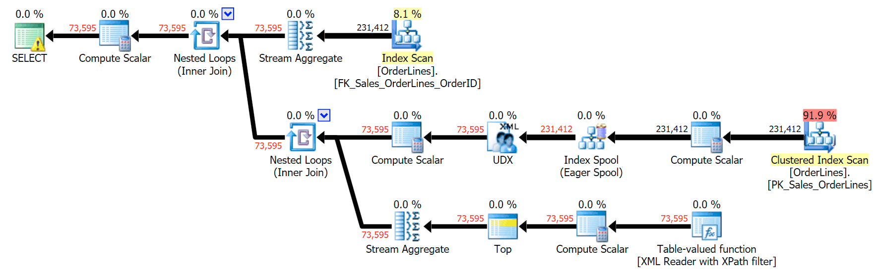
SELECT o.OrderID, OrderItems = STUFF((SELECT N'|' + Description
 FROM Sales.OrderLines
 WHERE OrderID = o.OrderID
 FOR XML PATH(N''), TYPE).value(N'text()[1]', N'nvarchar(max)'),1,1,N'')
FROM Sales.OrderLines AS o;
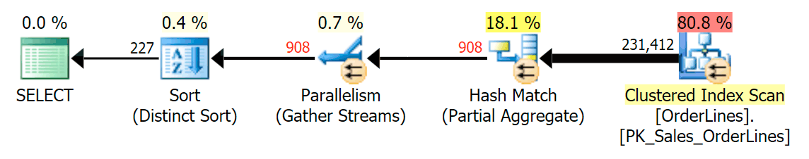
This is a typical query for solving this kind of problem, with the following execution plan (the warning in all of the plans is just for the implicit conversion coming out of the XPath filter):
However, it has a problem that you might notice in the output number of rows. You can certainly spot it when casually scanning the output:
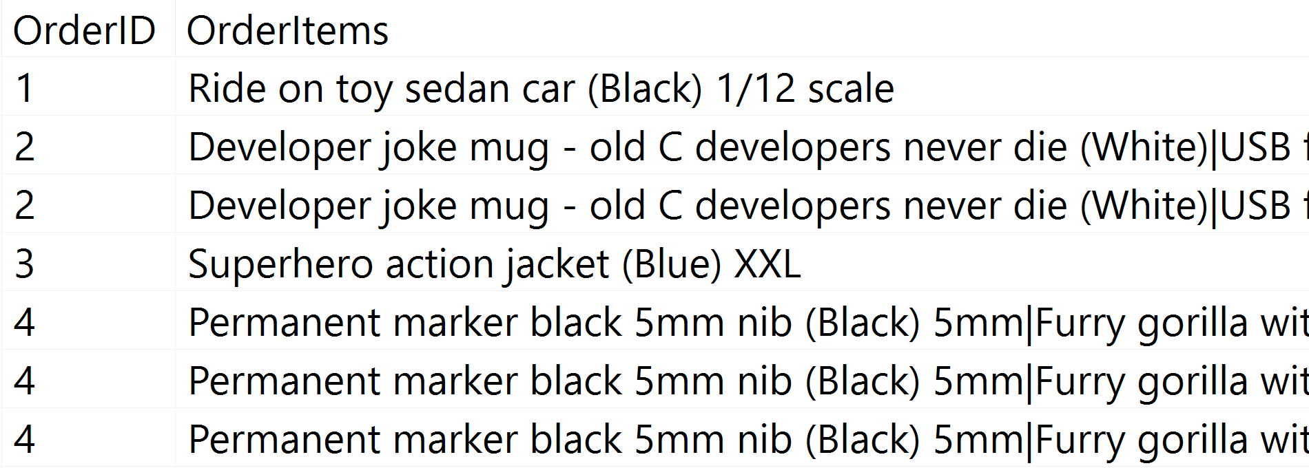
For every order, we see the pipe-delimited list, but we see a row for each item in each order. The knee-jerk reaction is to throw a DISTINCT on the column list:
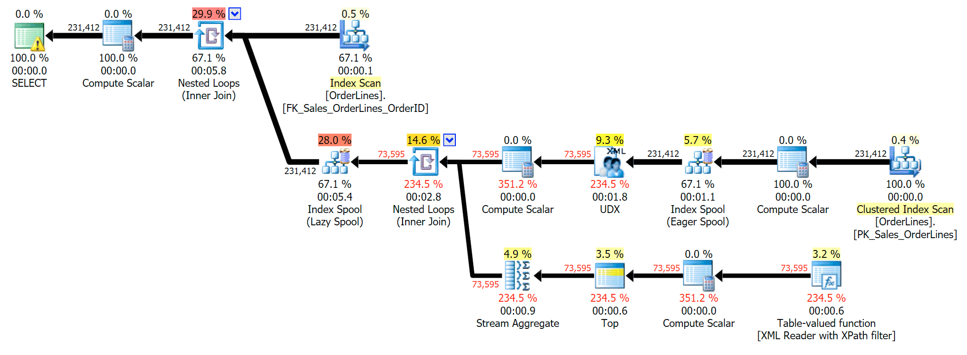
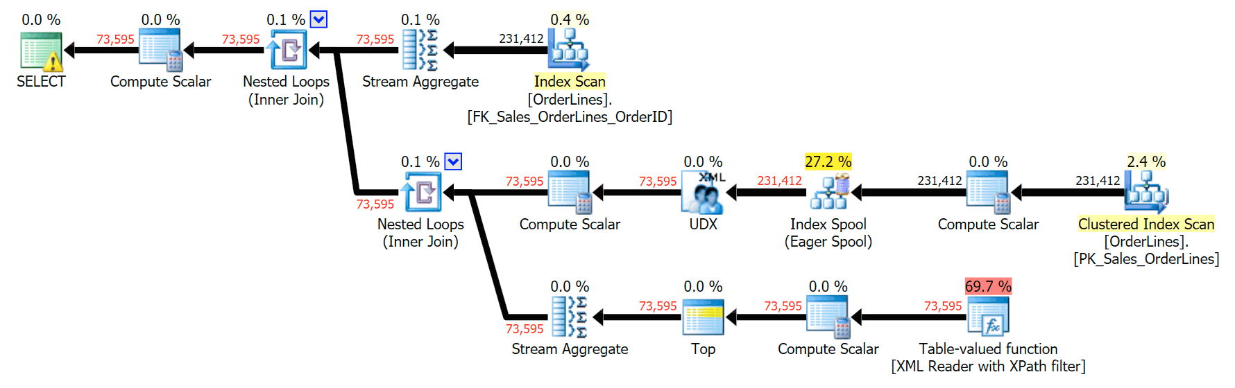
SELECT DISTINCT o.OrderID, OrderItems = STUFF((SELECT N'|' + Description
 FROM Sales.OrderLines
 WHERE OrderID = o.OrderID
 FOR XML PATH(N''), TYPE).value(N'text()[1]', N'nvarchar(max)'),1,1,N'')
FROM Sales.OrderLines AS o;
That eliminates the duplicates (and changes the ordering properties on the scans, so the results won't necessarily appear in a predictable order), and produces the following execution plan:
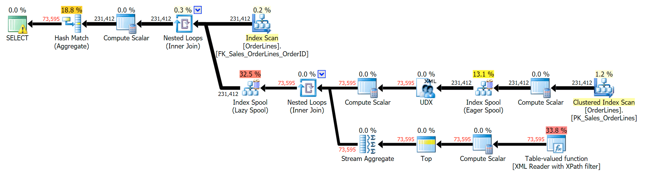
Another way to do this is to add a GROUP BY for the OrderID (since the subquery doesn't explicitly need to be referenced again in the GROUP BY):
SELECT o.OrderID, OrderItems = STUFF((SELECT N'|' + Description
 FROM Sales.OrderLines
 WHERE OrderID = o.OrderID
 FOR XML PATH(N''), TYPE).value(N'text()[1]', N'nvarchar(max)'),1,1,N'')
FROM Sales.OrderLines AS o
GROUP BY o.OrderID;
This produces the same results (though order has returned), and a slightly different plan:
The performance metrics, however, are interesting to compare.
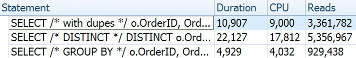
The DISTINCT variation took 4X as long, used 4X the CPU, and almost 6X the reads when compared to the GROUP BY variation. (Remember, these queries return the exact same results.)
We can also compare the execution plans when we change the costs from CPU + I/O combined to I/O only, a feature exclusive to Plan Explorer. We also show the re-costed values (which are based on the actual costs observed during query execution, a feature also only found in Plan Explorer). Here is the DISTINCT plan:
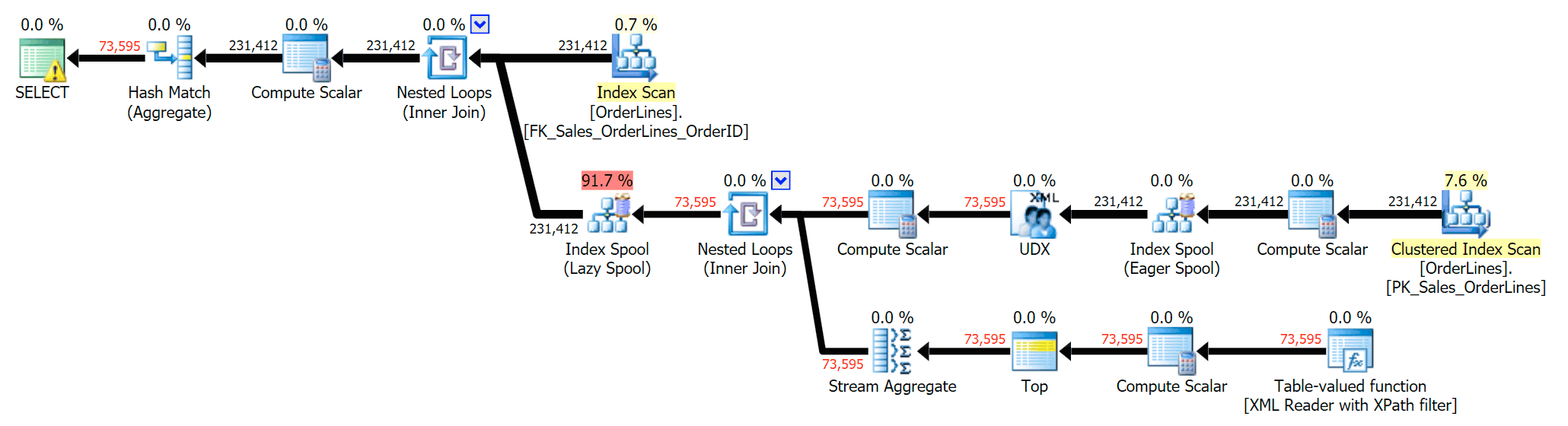
And here is the GROUP BY plan:
You can see that, in the GROUP BY plan, almost all of the I/O cost is in the scans (here's the tooltip for the CI scan, showing an I/O cost of ~3.4 "query bucks"). Yet in the DISTINCT plan, most of the I/O cost is in the index spool (and here's that tooltip; the I/O cost here is ~41.4 "query bucks"). Note that the CPU is a lot higher with the index spool, too. We'll talk about "query bucks" another time, but the point is that the index spool is more than 10X as expensive as the scan – yet the scan is still the same 3.4 in both plans. This is one reason it always bugs me when people say they need to "fix" the operator in the plan with the highest cost. Some operator in the plan will always be the most expensive one; that doesn't mean it needs to be fixed.
@AaronBertrand those queries are not really logically equivalent — DISTINCT is on both columns, whereas your GROUP BY is only on one
— Adam Machanic (@AdamMachanic) January 20, 2017
While Adam Machanic is correct when he says that these queries are semantically different, the result is the same – we get the same number of rows, containing exactly the same results, and we did it with far fewer reads and CPU.
So while DISTINCT and GROUP BY are identical in a lot of scenarios, here is one case where the GROUP BY approach definitely leads to better performance (at the cost of less clear declarative intent in the query itself). I'd be interested to know if you think there are any scenarios where DISTINCT is better than GROUP BY, at least in terms of performance, which is far less subjective than style or whether a statement needs to be self-documenting.
This post fit into my "surprises and assumptions" series because many things we hold as truths based on limited observations or particular use cases can be tested when used in other scenarios. We just have to remember to take the time to do it as part of SQL query optimization…
References
- Grouped Concatenation in SQL Server
- Grouped Concatenation : Ordering and Removing Duplicates
- Four Practical Use Cases for Grouped Concatenation
- SQL Server v.Next : STRING_AGG() performance
- SQL Server v.Next : STRING_AGG Performance, Part 2
The post Performance Surprises and Assumptions : GROUP BY vs. DISTINCT appeared first on SQLPerformance.com.
26 Jan 07:56

 [Advertisement]
Atalasoft’s imaging SDKs come with APIs & pre-built controls for web viewing, browser scanning, annotating, & OCR/barcode capture. Try it for 30 days with included support.
[Advertisement]
Atalasoft’s imaging SDKs come with APIs & pre-built controls for web viewing, browser scanning, annotating, & OCR/barcode capture. Try it for 30 days with included support.

Unstructured Data
by Remy Porter
Alex T had hit the ceiling with his current team, in terms of career advancement. He was ready to be promoted to a senior position, but there simply wasn’t room where he was- they were top-heavy as it was, and there were whispers among management of needing to make some cuts from that team. So Alex started looking for other openings.
There was another team at his company which had just lost all of its senior developers to other teams. Alex knew that was a bad sign, but in general, climbing the career ladder was a one-way street. Once he had a senior position, even if it was terrible, he could transfer to another team in a few months, keeping his senior title and salary.
Perry was the team’s technical director. “I’ve been laying out the TPM architecture for years,” Perry explained, “and you are going to be part of implementing my vision.” That vision was an Internal Framework called “Total Process Management”, which, as the name implied, was a flexible business rules engine that would manage all of their business processes, from HR, to supply chain, to marketing, it would do everything. “We’re bringing the latest technologies to bear, it’ll be based on RESTful microservices with a distributed backend. But we need to staff up to achieve this, so we’re going to be doing a lot of interviews over the next few months, you and me.”
Alex knew he could apply for another internal transfer after six months. He already saw this was a disaster, the only question was how disastrous would it be?
While the code Perry had him writing was an overcomplicated mess of trendy ideas badly implemented, the worst part was doing the interviews. Perry sat in on every phase of the interview, and had Opinions™ about everything the candidate had on their resume.
“You used Angular for that?” he demanded from one candidate, sneering, and drawing a bright red “X” on their resume. He criticized another for using a relational database when they could have used MongoDB. One interview ended early when the candidate admitted that they didn’t spend their nights and weekends hacking at personal projects.
The worst part, for Alex, was his role in the technical screens. He’d read about the failures of white-board programming, the uselessness of asking trivia questions: “How do you reverse a linked-list?” wasn’t exactly a great interview question. He’d planned out a set of questions he thought would be better, and even some hands-on coding, but Perry nixed that.
“I want you to build a test with an answer key,” Perry said. “Because at some point, we may want to have non-technical people doing a first-pass screening as our team grows and more people want to join it. Use that in the technical portion of the interview.”
Interviews turned into days, days turned into weeks, weeks into months, and eventually Perry brought in Jack. Jack had worked at Google (as an intern), and Perry loved that. In fact, through the whole interview, Perry and Jack got on like a house on fire, smiling, laughing, happily bashing the same technologies and waxing rhapsodic over the joys of using Riak (Mongo was so last year, they were junking all of their database access to use Riak now).
Eventually, Perry left and it was Alex’s turn to recite his test, and compare the results against his answer key. “What’s a linked-list?” he asked, dying on the inside.

“It’s a navigation widget on websites.”
Alex blinked, but continued. “How does a linked-list differ from a doubly-linked-list?”
“A doubly-linked list has a pop-up menu so you can have more links in the list,” Jack said.
For the first time since he’d written his test, Alex was actually excited to see the results. Jack wasn’t just wrong, he was finding incredibly new ways to be wrong. He claimed a binary-tree was a kind of legacy hard-drive. Or RAM, perhaps, it wasn’t really clear from his answer. Design Patterns were templates you could use… in Photoshop.
Alex thanked Jack for his time, sent him on his way, and then went to compare notes with Perry.
Perry was positively beaming. “I think we found a really great candidate,” he said. “Jack’s sharp as a tack, and is definitely a culture fit. What did you think?”
“Well,” Alex started, and then stopped. Perry was difficult to handle, so Alex decided that he should be as diplomatic as possible. “It started pretty well, but when we started talking about data-structures- he was really weak. It’s a bad sign. We should pass.”
“That’s probably not a big deal,” Perry said, “I don’t care if he knows Oracle or not. We use unstructured data.”
[Advertisement]
Atalasoft’s imaging SDKs come with APIs & pre-built controls for web viewing, browser scanning, annotating, & OCR/barcode capture. Try it for 30 days with included support.
26 Jan 07:52
 [Advertisement] Manage IT infrastructure as code across all environments with Puppet. Puppet Enterprise now offers more control and insight, with role-based access control, activity logging and all-new Puppet Apps. Start your free trial today!

Predict Correct
by Ellis Morning

Steven was an engineer at a US-based company whose leadership had decided to take some dramatic cost-saving measures. A mandatory company meeting convened at 12:00PM, with nary a crumb of food in sight, to allow management to make their big announcement:
"We're opening an office offshore, and one of the first things we'll be transitioning there is product documentation."
Ah, transitioning: a nice way to say they were firing every US-based tech writer immediately. From that point forward, the engineers would have to send notes on product features to the offshore team, who would then compile the documentation.
Steven was nervous about the prospect. He'd had a good working relationship with the tech writers. They could take his notes, add their personal experiences with the products, and compile it all into something useful (for the rare user who actually bothered to look at the manuals). Hesitantly, he raised his hand. "Will the offshore team be trained on our products?"
"Don't worry. We're working with a consulting company that's helping us hire the best talent available," the meeting presenter assured him with a saccharine smile.
In other words, No way in hell. Steven saw through the ruse, but didn't have the guts to call it out. No one else did, either. After all, no one wanted to give management the idea that perhaps engineers were just as replaceable as tech writers.
They had no choice but to wait and see. With any luck, the hiring firm would find some good writers, at least.
A few weeks later, Steven sent off his first round of notes and crossed his fingers. Unfortunately, what he got back was his own notes copied and pasted into the standard manual template, surrounded with typos and broken English.
No, wait, they hadn't just copied his notes. They'd tried to "improve" upon them. In one case where Steven explained the behavior of a quirky installer, he'd written:
The installer doesn't always guess right about the drive.
The mangled sentence that had limped back from the foreign office read:
The installer doesn't always predict correct the drive.
There were also problems with fonts, indentation, tables, lists—practically every aspect of formatting. Strange, because the offshore techs were supposed to be working with software that handled all the layout and formatting details for them.
Steven's documentation wasn't the only example of this problem. Together, the concerned engineers banded together and demanded face-time with management.
"I give foreign English speakers a lot of credit. I'm happy to cut them slack," Steven said once he and others had presented the shoddy documentation. "But if your job is to write English, then you kinda need to understand English spelling, grammar, and idiomatic phrasing. Documentation is the one chance we have to inform users of what they need to know so they don't go off the rails. Offshoring may be cheaper in the short run, but with docs like these, we're gonna end up with a lot more support calls and unhappy customers."
Steven then summoned the bravery that'd eluded him during the initial lunch meeting. "There's no point sending text to the other side of the planet to be pasted into the layout, just so we can clean up the mess they send back. I say we generate the user manuals ourselves and cut out the middleman."
The upper manager squirmed in his chair during an uncomfortable pause. "I see your point. But the user manuals are generated with complicated layout software. This thing has a steep learning curve and big per-seat licensing fees. There's no way we can arrange for the onshore engineering team to use it."
So the documentation text had to be round-tripped through the foreign office. Even when the engineers sent off complete final drafts, they always came back with changes—for the worse. Were the offshore techs bored? Struggling to justify their existence? Whatever the case, Steven and others had to slog through their manuals line by line, marking up errors, and sending them back to be fixed. Maybe.
Once upon a time, the company had paid for quality documentation with US tech writer wages. Now they paid for inferior documentation with sweat, tears, torn hair, US engineer wages, and offshore tech wages. Not quite the savings their leadership had envisioned.
<SHAMELESS PLUG> I've finished the second book in my Sword and Starship series! Harbingers is the direct sequel to Blood's Force. If you like fantasy in your sci-fi (or is it sci-fi in your fantasy?), go check it out at Amazon, iBooks, Kobo, or Nook. </SHAMELESS PLUG>
[Advertisement] Manage IT infrastructure as code across all environments with Puppet. Puppet Enterprise now offers more control and insight, with role-based access control, activity logging and all-new Puppet Apps. Start your free trial today!
26 Jan 07:35

Pure Storage’s FlashBlade is now GA
by Dave Henry
I wrote about FlashBlade when it was first announced in 2016. At the time I was very excited about the possibilities of this platform. I wasn’t able to get hands-on with the platform. The closest I got was being able to hold and examine one of the blades — encased in a Lucite box. (Really. They handed it to me all boxed up. I was tempted to use my multitool to open the box up to conduct a more-thorough examination, but not only did it feel like it would be rude, they also seemed to always make sure I was within arms-reach of at least three Pure employees at any point the blade was within arms-reach of me… (Kudos to them on having done their advance research.)) At that time, not all of the specifications had been solidified, but those details are available now. What It Is
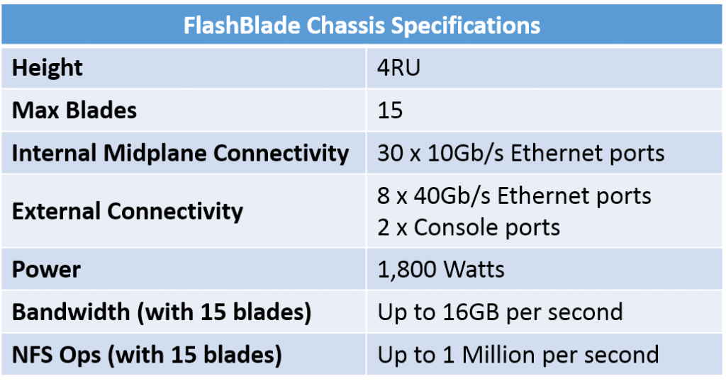
Each FlashBlade chassis is 4RU tall and can hold up to 15 blades. With Elasticity 1.2, FlashBlade storage can be one or two chassis (up to 30 blades). Future releases will allow for greater numbers of chassis (I’m pretty sure that “chassis” is the plural of “chassis”…) to be combined together. The blades come in two sizes: 8.8TB or 52TB of raw Flash storage, allowing for up to 780TB of raw Flash storage in a single chassis. Blades of differing capacities can be installed in the same chassis. Elasticity uses inline data compression to allow for a higher effective capacity. Elasticity does not currently do data deduplication, although it’s on the roadmap for a future release. Each blade uses super-low-latency PCIe to connect the Flash chips to the blade’s processors. Blades within a chassis use an internal 10Gb Ethernet midplane for inter-blade communication. Communication between chassis occurs over the external 40Gb Ethernet ports. Chassis SpecsThe FlashBlade chassis specifications are below.
AvailabilityFlashBlade and Elasticity 1.2 are available starting today. FuturesAs of this writing, Elasticity only offers NFSv3 file access. SMB file access is currently in Beta test. S3 object access is planned to start Beta in February. GeekFluent’s ThoughtsI only have two thoughts on this announcement:
|

26 Jan 07:35

My Interview with Geek Whisperers on Being a Technical Generalist
by Dave Henry
I know this will cause my long-time readers to immediately ask two questions:
I’ll attempt to answer these questions as best I can.
It was a great conversation that I enjoyed a lot. My job search was more of a tangent that got a mention. What we focused on was the idea of being a technical generalist (as opposed to specializing in one particular area), and where (and how) this can be either an advantage or disadvantage to one’s career. Having been working full-time in IT for 30 years now (and a year and half part-time prior to that), I’ve been a generalist in simple-job-description-defying hybrid roles for the vast majority of my career — most often by choice, but sometimes having it thrust upon me due to circumstances. During the course of the podcast, we discuss this and the advantages and pitfalls of this approach to one’s career, as well as a number of related topics and stories. Oh, and I also received the Official Geek Whisperers confirmation of my Unicorn Status. (You’ll have to listen to the episode to understand this…) You can check out the podcast episode here. Give it a listen, then let me know what you think, or ask any follow-on questions, in the comments below. Thanks to Amy Lewis, John Mark Troyer, and Matt Broberg for inviting me on! Let’s not wait another 128 episodes before we do this again… |
26 Jan 07:34


Microsoft Products vs Hadoop/OSS Products
by James Serra
Microsoft’s end goal is for Azure to become the best cloud platform for customers to run their data workloads. This means Microsoft will provide customers the best environment to run their big data/Hadoop as well as a place where Microsoft can offer services with our unique point-of-view. Specific decision points on using Hadoop is if the customer wants to use open source technologies or not. Some of the benefits of running open source software (OSS) on Azure include:
- Quick installs
- Support
- Easy scale
- Products work together
- Don’t need to get your own hardware
To determine the cost savings by moving your OSS to Azure, see the Total Cost of Ownership (TCO) Calculator.
Of course there are many benefits of using Microsoft products over OSS, such as ease of use, support, better security, easier to find people with skills, less frequent version updates, more stable (less bugs), more compatibility and integration between products, etc. But there are still reasons to use OSS (i.e. cost, faster performance in some cases, more product selection and features), so I created a list that shows many of the Microsoft products and their equivalent, or close equivalent, Hadoop/OSS product.
I tried to list only Apache products unless there was no equivalent Apache product or there is a really popular Open Source Software (OSS) product.
| Microsoft Product | Hadoop/Open Source Software Product |
| Office365/Excel | OpenOffice/Calc |
| DocumentDB | MongoDB, MarkLogic, HBase, Cassandra |
| SQL Database | SQLite, MySQL, PostgreSQL, MariaDB |
| Azure Data Lake Analytics/YARN | None |
| Azure VM/IaaS | OpenStack |
| Blob Storage | HDFS, Ceph (Note: These are distributed file systems and Blob storage is not distributed) |
| Azure HBase | Apache HBase (Azure HBase is a service wrapped around Apache HBase), Apache Trafodion |
| Event Hub | Apache Kafka |
| Azure Stream Analytics | Apache Storm, Apache Spark, Twitter Heron |
| Power BI | Apache Zeppelin, Apache Jupyter, Airbnb Caravel, Kibana |
| HDInsight | Hortonworks (pay), Cloudera (pay), MapR (pay) |
| Azure ML | Apache Mahout, Apache Spark MLib |
| Microsoft R Open | R |
| SQL Data Warehouse | Apache Hive, Apache Drill, Presto |
| IoT Hub | Apache NiFi |
| Azure Data Factory | Apache Falcon, Airbnb Airflow |
| Azure Data Lake Storage/WebHDFS | HDFS Ozone |
| Azure Analysis Services/SSAS | Apache Kylin, AtScale (pay) |
| SQL Server Reporting Services | None |
| Hadoop Indexes | Jethro Data (pay) |
| Azure Data Catalog | Apache Atlas |
| PolyBase | Apache Drill |
| Azure Search | Apache Solr, Apache ElasticSearch (Azure Search build on ES) |
| Others | Apache Flink, Apache Ambari, Apache Ranger, Apache Knox |
Many of the Hadoop/OSS products are available in Azure. If you feel I’m missing some products from this list, please let me know as this is very subjective and comments are always welcome!
26 Jan 07:34

Code to show rolled back transactions after a crash
by Paul Randal
In Monday’s Insider newsletter I discussed an email question I’d been sent about how to identify the transactions that had rolled back because of a crash, and I said I’d blog some code to do it.
First of all you need to know the time of the crash. We can’t get this exactly (from SQL Server) unless SQL Server decides to shut itself down for some reason (like tempdb corruption) but we can easily get the time that SQL Server restarted, which is good enough, as we just need to know a time that’s after the transactions started before the crash, and before those transactions finished rolling back after a crash. We can get the startup time from the sqlserver_start_time column in the output from sys.dm_os_sys_info.
Then we can search in the transaction log, using the fn_dblog function, for LOP_BEGIN_XACT log records from before the crash point that have a matching LOP_ABORT_XACT log record after the crash point, and with the same transaction ID. This is easy because for LOP_BEGIN_XACT log records, there’s a Begin Time column, and for LOP_ABORT_XACT log records (and, incidentally, for LOP_COMMIT_XACT log records), there’s an End Time column in the TVF output.
And there’s a trick you need to use: to get the fn_dblog function to read log records from before the log clears (by the checkpoints that crash recovery does, in the simple recovery model, or by log backups, in other recovery models), you need to enable trace flag 2537. Now, if do all this too long after crash recovery runs, the log may have overwritten itself and so you won’t be able to get the info you need, but if you’re taking log backups, you could restore a copy of the database to the point just after crash recovery has finished, and then do the investigation.
After that, the tricky part is matching what those transactions were doing back to business operations that your applications were performing. If you don’t name your transactions, that’s going to be pretty hard, as all you’ve got are the generic names that SQL Server gives transactions (like INSERT, DELETE, DROPOBJ). Whatever the reason you might want this information, your applications should be written so they gracefully handle transaction failures and leave the database in a consistent state (as far as your business rules are concerned – of course SQL Server leaves the database in a transactionally-consistent state after a crash).
I’ve written some code and encapsulated it in a proc, sp_SQLskillsAbortedTransactions, which is shown in full at the end of the post. To use it, you go into the context of the database you’re interested in, and just run the proc. It takes care of enabling and disabling the trace flag.
Here’s an example of a crash situation and using the proc.
First I’ll create a table and start a transaction:
USE [master];
GO

IF DATABASEPROPERTYEX (N'Company', N'Version') > 0
BEGIN
    ALTER DATABASE [Company] SET SINGLE_USER WITH ROLLBACK IMMEDIATE;
    DROP DATABASE [Company];
END
GO

CREATE DATABASE [Company];
GO
USE [Company];
GO

CREATE TABLE [test] ([c1] INT, [c2] INT, [c3] INT);
GO
INSERT INTO [test] VALUES (0, 0, 0);
GO

BEGIN TRAN FirstTransaction;
INSERT INTO [Test] VALUES (1, 1, 1);
GO
Now in a second window, I’ll start another transaction, and force the log to flush to disk (as I haven’t generated enough log to have the current log block automatically flush to disk):
USE [Company];
GO

BEGIN TRAN SecondTransaction;
INSERT INTO [Test] VALUES (2, 2, 2);
GO

EXEC sp_flush_log;
GO
And in a third window, I’ll force a crash:
SHUTDOWN WITH NOWAIT;
GO
After restarting the instance, I can use this code to run my proc:
USE [Company];
GO

EXEC sp_SQLskillsAbortedTransactions;
GO
Begin Time               Transaction Name   Started By       Transaction ID
------------------------ ------------------ ---------------- --------------
2017/01/18 17:09:36:190  FirstTransaction   APPLECROSS\Paul  0000:00000374
2017/01/18 17:09:40:600  SecondTransaction  APPLECROSS\Paul  0000:00000375
Cool eh?
Here’s the code – enjoy!
/*============================================================================
  File:     sp_SQLskillsAbortedTransactions.sql

  Summary:  This script cracks the transaction log and shows which
            transactions were rolled back after a crash

  SQL Server Versions: 2012 onwards
------------------------------------------------------------------------------
  Written by Paul S. Randal, SQLskills.com

  (c) 2017, SQLskills.com. All rights reserved.

  For more scripts and sample code, check out
    http://www.SQLskills.com

  You may alter this code for your own *non-commercial* purposes. You may
  republish altered code as long as you include this copyright and give due
  credit, but you must obtain prior permission before blogging this code.

  THIS CODE AND INFORMATION ARE PROVIDED "AS IS" WITHOUT WARRANTY OF
  ANY KIND, EITHER EXPRESSED OR IMPLIED, INCLUDING BUT NOT LIMITED
  TO THE IMPLIED WARRANTIES OF MERCHANTABILITY AND/OR FITNESS FOR A
  PARTICULAR PURPOSE.
============================================================================*/

USE [master];
GO

IF OBJECT_ID (N'sp_SQLskillsAbortedTransactions') IS NOT NULL
    DROP PROCEDURE [sp_SQLskillsAbortedTransactions];
GO

CREATE PROCEDURE sp_SQLskillsAbortedTransactions
AS
BEGIN
    SET NOCOUNT ON;

    DBCC TRACEON (2537);

    DECLARE @BootTime	DATETIME;
    DECLARE @XactID     CHAR (13);

    SELECT @BootTime = [sqlserver_start_time] FROM sys.dm_os_sys_info;

    IF EXISTS (SELECT * FROM [tempdb].[sys].[objects]
        WHERE [name] = N'##SQLskills_Log_Analysis')
        DROP TABLE [##SQLskills_Log_Analysis];

    -- Get the list of started and rolled back transactions from the log
    SELECT
        [Begin Time],
        [Transaction Name],
        SUSER_SNAME ([Transaction SID]) AS [Started By],
        [Transaction ID],
        [End Time],
        0 AS [RolledBackAfterCrash],
        [Operation]
    INTO ##SQLskills_Log_Analysis
    FROM fn_dblog (NULL, NULL)
    WHERE ([Operation] = 'LOP_BEGIN_XACT' AND [Begin Time] < @BootTime) OR ([Operation] = 'LOP_ABORT_XACT' AND [End Time] > @BootTime);

    DECLARE [LogAnalysis] CURSOR FAST_FORWARD FOR
    SELECT
        [Transaction ID]
    FROM
        ##SQLskills_Log_Analysis;

    OPEN [LogAnalysis];

    FETCH NEXT FROM [LogAnalysis] INTO @XactID;

    WHILE @@FETCH_STATUS = 0
    BEGIN
        IF EXISTS (
            SELECT [End Time] FROM ##SQLskills_Log_Analysis
            WHERE [Operation] = 'LOP_ABORT_XACT' AND [Transaction ID] = @XactID)
        UPDATE ##SQLskills_Log_Analysis SET [RolledBackAfterCrash] = 1
            WHERE [Transaction ID] = @XactID
            AND [Operation] = 'LOP_BEGIN_XACT';

        FETCH NEXT FROM [LogAnalysis] INTO @XactID;
    END;

    CLOSE [LogAnalysis];
    DEALLOCATE [LogAnalysis];

    SELECT
        [Begin Time],
        [Transaction Name],
        [Started By],
        [Transaction ID]
    FROM ##SQLskills_Log_Analysis
    WHERE [RolledBackAfterCrash] = 1;

    DBCC TRACEOFF (2537);

    DROP TABLE ##SQLskills_Log_Analysis;
END
GO

EXEC sys.sp_MS_marksystemobject [sp_SQLskillsAbortedTransactions];
GO

-- USE [Company]; EXEC sp_SQLskillsAbortedTransactions;
The post Code to show rolled back transactions after a crash appeared first on Paul S. Randal.
26 Jan 07:33
Don’t Call it a Data Lake, its a Data River. Here’s Why.
by Stefan Groschupf
Click to learn more about video blogger Stefan Groschupf. Introducing the Big Data & Brews video blog series presented by Stefan Groschupf, Founder of Datameer. The series will touch on hot topics within the business of Big Data, Machine Learning, Analytics, Internet of Things, Cloud Computing, Data Lakes, Data Governance, Modern BI, NoSQL and Next Generation Technologies. […]
The post Don’t Call it a Data Lake, its a Data River. Here’s Why. appeared first on DATAVERSITY.
26 Jan 07:32
Announcing the SQL Server v.Next Early Adoption Program
by SQL Server Team
This post was authored by Anna Shrestinian, Program Manager, SQL Server
What is the SQL Server Early Adoption Program (SQL EAP)?
The SQL Server Early Adoption Program (SQL EAP) is a Microsoft program started in January 2017 to help both customers and partners adopt the next version of SQL Server before general availability.
Who is SQL EAP for?
If you are interested in adopting SQL Server v.Next on Windows or Linux in production, then SQL EAP is for you. SQL EAP is also for partners who want to build SI (system integrator) offerings and ISV (independent software vendor) applications using SQL Server v.Next. Upon successful validation, these applications and solutions can be supported in production prior to the general availability release. Customers and partners who would like to validate new features such as Adaptive Query Processing and High Availability (HA) on Linux are an especially good fit for SQL EAP. Enroll for the program here.
What are the benefits?
- Through the program you will have direct access to the engineering team through a Program Manager Buddy. Your PM Buddy is there as a primary contact within the development team to help connect you to the right people to help your solution adopt SQL Server v.Next. Typically, PM Buddies communicate with the customer via email and regularly scheduled meetings. PM Buddies help scope the project when the customer first joins SQL EAP so that there is common understanding of the schedule and requirements.
- SQL EAP participants have the opportunity to bring your workload to the SQL Customer Advisory Team Customer Lab to directly engage and test with the SQL Server team.
- Customers in SQL EAP will be able to try out new features, sometimes before the public gets to see them, and provide the feedback directly to the engineering team. They will have the opportunity to provide input into the prioritization of product requirements for SQL Server v.Next via regular surveys. Participants will also be able to discuss feature design with PMs.
- You will have access to a private Yammer group for SQL EAP customers to communicate with one another and the engineering team, helping customers learn from each other. Content on the private Yammer group will be considered confidential and covered by the Microsoft NDA required to participate in SQL EAP.
- Customers going into production will be fully supported by Microsoft Support before general availability. A special support channel is provided to raise cases for SQL Server v.Next. The SQL Server engineering team will be backing up the Microsoft Support team to provide assistance as needed. Customers in production will also have support for release-to-release upgrades.
What are the requirements?
- Complete the form here. Enrollments will be evaluated and a PM Buddy aligned to access workload validation and those on track for production deployments.
- An NDA with Microsoft will be required to participate in the program. If you do not already have an NDA, we will help to get one signed.
- Customers in SQL EAP that are going in production will need to sign a EULA amendment that grants them the permission to use the software in production.
Get Started Today:
Apply for the program here!
Join the Webinar:
We are having a webinar called SQL Server on Linux Next Steps on 1/24 at 6pm PST and also 1/31 at 6pm PST. Please join us to learn more about SQL Early Adoption Program. The webinar covers:
- The latest updates to SQL Server v.Next
- How SQL Server 2016 v.Next can improve your applications and solutions
- Our SQL Early Adoption Program where you can get advice from our technical experts and get technical resources to help upgrade or migrate your applications to SQL Server v.Next.
We will have a Q&A session at the end of the webinar.
Link to Skype Broadcast 1/24 at 6pm PST
Link to Skype Broadcast 1/31 at 6pm PST
Learn More:
26 Jan 07:32
SQL Server next version CTP 1.2 now available
by SQL Server Team
As part of our rapid preview model, Microsoft is excited to announce that the next version of SQL Server (SQL Server v.Next) Community Technology Preview (CTP) 1.2 is now available on both Windows and Linux. In CTP 1.2 we implemented bug fixes and added support for SQL Server v.Next on SUSE Linux Enterprise Server. You can try the preview in your development and test environments now, or apply to join the SQL Server Early Adoption Program to get support for implementing SQL Server v.Next in production.
Key CTP 1.2 enhancement: Support for SUSE Linux Enterprise
In SQL Server v.Next, a key design principle has been to provide customers with choice about how to develop and deploy SQL Server applications: using technologies they love like Java, .NET, PHP, Python, R and Node.js, all on the platform of their choosing. Now in CTP 1.2, Microsoft is bringing the power of SQL Server to SUSE Linux Enterprise Server, providing more deployment options and a streamlined acquisition process.
Said Kristin Kinan, Global Alliance Director, Public Cloud at SUSE, “We’re thrilled that Microsoft is announcing support for SQL Server v.Next on SUSE Linux Enterprise Linux. SQL Server and SUSE customers will now be able to run performant, secured SQL Server applications with reliable, cost-effective infrastructure from SUSE.”
You can get started with SQL Server on SUSE Linux Enterprise Server v12 SP2 using the installation directions. To learn more about how SQL Server runs on SUSE Linux Enterprise Server and container platforms, you can register for this upcoming webinar that will take place on February 15, 2017. For additional detail on CTP 1.2, please visit What’s New in SQL Server v.Next, Release Notes and Linux documentation.
SQL Server Early Adoption Program (EAP)
Today we also announced the SQL Server v.Next Early Adoption Program (EAP). The Early Adoption Program is designed to help customers and partners evaluate new features in SQL Server v.Next, and to build and deploy applications for SQL Server v.Next on Windows and Linux. Qualified applicants will receive technical assistance from Microsoft engineers to deploy and support an application in production before general availability, or to build or modernize an application for SQL Server v.Next. Read the detailed blog on EAP to learn more about all the benefits of this program and how to get started.
Get SQL Server v.Next CTP 1.2 today!
Try the preview of the next release of SQL Server today! Get started with the preview of SQL Server with our developer tutorials that show you how to install and use SQL Server v.Next on macOS, Docker, Windows, and Linux and quickly build an app in a programming language of your choice.
- Sign up for the Early Adoption Program (EAP)
- Install on SUSE Linux Enterprise Server
- Install on Red Hat Enterprise Linux
- Install on Ubuntu Linux
- Pull and run a Docker container on Linux, Windows, or macOS
- Download the preview for Windows
- Create a SQL Server on Linux virtual machine in Azure
- Register for the Introduction to SQL Server on SUSE Linux Enterprise Server Webinar
Have questions? Join the discussion of SQL Server v.Next at MSDN. If you run into an issue or would like to make a suggestion, you can let us know through Connect. We look forward to hearing from you!
26 Jan 07:32
Compression and its Effects on Performance
by Erin Stellato
One of the many new features introduced back in SQL Server 2008 was Data Compression. Compression at either the row or page level provides an opportunity to save disk space, with the trade off of requiring a bit more CPU to compress and decompress the data. It's frequently argued that the majority of systems are IO-bound, not CPU-bound, so the trade off is worth it. The catch? You had to be on Enterprise Edition to use Data Compression. With the release of SQL Server 2016 SP1, that has changed! If you're running Standard Edition of SQL Server 2016 SP1 and higher, you can now use Data Compression. There's also a new built-in function for compression, COMPRESS (and its counterpart DECOMPRESS). Data Compression does not work on off-row data, so if you have a column like NVARCHAR(MAX) in your table with values typically more than 8000 bytes in size, that data won't be compressed (thanks Adam Machanic for that reminder). The COMPRESS function solves this problem, and compresses data up to 2GB in size. Moreover, while I'd argue that the function should only be used for large, off-row data, I thought comparing it directly against row and page compression was a worthwhile experiment.
SETUP
For test data, I'm working from a script Aaron Bertrand has used previously, but I've made some tweaks. I created a separate database for testing but you can use tempdb or another sample database, and then I started with a Customers table that has three NVARCHAR columns. I considered creating larger columns and populating them with strings of repeating letters, but using readable text gives a sample that's more realistic and thus provides greater accuracy.
Note: If you're interested in implementing compression and want to know how it will affect storage and performance in your environment, I HIGHLY RECOMMEND THAT YOU TEST IT. I'm giving you the methodology with sample data; implementing this in your environment shouldn't involve additional work.
You'll note below that after creating the database we're enabling Query Store. Why create a separate table to try and track our performance metrics when we can just use functionality built-in to SQL Server?!
USE [master];
GO

CREATE DATABASE [CustomerDB]
 CONTAINMENT = NONE
 ON  PRIMARY
 (
   NAME = N'CustomerDB', FILENAME = N'C:\Databases\CustomerDB.mdf' ,
   SIZE = 4096MB , MAXSIZE = UNLIMITED, FILEGROWTH = 65536KB
 )
 LOG ON
 (
   NAME = N'CustomerDB_log', FILENAME = N'C:\Databases\CustomerDB_log.ldf' ,
   SIZE = 2048MB , MAXSIZE = UNLIMITED , FILEGROWTH = 65536KB
 );
GO

ALTER DATABASE [CustomerDB] SET COMPATIBILITY_LEVEL = 130;
GO
ALTER DATABASE [CustomerDB] SET RECOVERY SIMPLE;
GO
ALTER DATABASE [CustomerDB] SET QUERY_STORE = ON;
GO
ALTER DATABASE [CustomerDB] SET QUERY_STORE
(
  OPERATION_MODE = READ_WRITE,
  CLEANUP_POLICY = (STALE_QUERY_THRESHOLD_DAYS = 30),
  DATA_FLUSH_INTERVAL_SECONDS = 60,
  INTERVAL_LENGTH_MINUTES = 5,
  MAX_STORAGE_SIZE_MB = 256,
  QUERY_CAPTURE_MODE = ALL,
  SIZE_BASED_CLEANUP_MODE = AUTO,
  MAX_PLANS_PER_QUERY = 200
);
GO
Now we'll set up some things inside the database:
USE [CustomerDB];
GO
ALTER DATABASE SCOPED CONFIGURATION SET MAXDOP = 0;
GO

-- note: I removed the unique index on [Email] that was in Aaron's version
CREATE TABLE [dbo].[Customers]
(
	[CustomerID] [int] NOT NULL,
	[FirstName] [nvarchar](64) NOT NULL,
	[LastName] [nvarchar](64) NOT NULL,
	[EMail] [nvarchar](320) NOT NULL,
	[Active] [bit] NOT NULL DEFAULT 1,
	[Created] [datetime] NOT NULL DEFAULT SYSDATETIME(),
	[Updated] [datetime] NULL,
  CONSTRAINT [PK_Customers] PRIMARY KEY CLUSTERED ([CustomerID])
);
GO

CREATE NONCLUSTERED INDEX [Active_Customers]
ON [dbo].[Customers]([FirstName],[LastName],[EMail])
WHERE ([Active]=1);
GO

CREATE NONCLUSTERED INDEX [PhoneBook_Customers]
ON [dbo].[Customers]([LastName],[FirstName])
INCLUDE ([EMail]);
With the table created, we'll add some data, but we're adding 5 million rows instead of 1 million. This takes about eight minutes to run on my laptop.
INSERT dbo.Customers WITH (TABLOCKX)
  (CustomerID, FirstName, LastName, EMail, [Active])
  SELECT rn = ROW_NUMBER() OVER (ORDER BY n), fn, ln, em, a
  FROM
  (
    SELECT TOP (5000000) fn, ln, em, a = MAX(a), n = MAX(NEWID())
    FROM
    (
      SELECT fn, ln, em, a, r = ROW_NUMBER() OVER (PARTITION BY em ORDER BY em)
      FROM
      (
        SELECT TOP (20000000)
          fn = LEFT(o.name,  64),
          ln = LEFT(c.name,  64),
          em = LEFT(o.name,  LEN(c.name)%5+1) + '.'
             + LEFT(c.name,  LEN(o.name)%5+2) + '@'
             + RIGHT(c.name, LEN(o.name + c.name)%12 + 1)
             + LEFT(RTRIM(CHECKSUM(NEWID())),3) + '.com',
          a  = CASE WHEN c.name LIKE '%y%' THEN 0 ELSE 1 END
        FROM sys.all_objects AS o CROSS JOIN sys.all_columns AS c
        ORDER BY NEWID()
      ) AS x
    ) AS y WHERE r = 1
    GROUP BY fn, ln, em
    ORDER BY n
  ) AS z
  ORDER BY rn;
GO
Now we'll create three more tables: one for row compression, one for page compression, and one for the COMPRESS function. Note that with the COMPRESS function, you must create the columns as VARBINARY data types. As a result, there are no nonclustered indexes on the table (as you cannot create an index key on a varbinary column).
CREATE TABLE [dbo].[Customers_Page]
(
	[CustomerID] [int] NOT NULL,
	[FirstName] [nvarchar](64) NOT NULL,
	[LastName] [nvarchar](64) NOT NULL,
	[EMail] [nvarchar](320) NOT NULL,
	[Active] [bit] NOT NULL DEFAULT 1,
	[Created] [datetime] NOT NULL DEFAULT SYSDATETIME(),
	[Updated] [datetime] NULL,
  CONSTRAINT [PK_Customers_Page] PRIMARY KEY CLUSTERED ([CustomerID])
);
GO

CREATE NONCLUSTERED INDEX [Active_Customers_Page]
ON [dbo].[Customers_Page]([FirstName],[LastName],[EMail])
WHERE ([Active]=1);
GO

CREATE NONCLUSTERED INDEX [PhoneBook_Customers_Page]
ON [dbo].[Customers_Page]([LastName],[FirstName])
INCLUDE ([EMail]);
GO

CREATE TABLE [dbo].[Customers_Row]
(
	[CustomerID] [int] NOT NULL,
	[FirstName] [nvarchar](64) NOT NULL,
	[LastName] [nvarchar](64) NOT NULL,
	[EMail] [nvarchar](320) NOT NULL,
	[Active] [bit] NOT NULL DEFAULT 1,
	[Created] [datetime] NOT NULL DEFAULT SYSDATETIME(),
	[Updated] [datetime] NULL,
  CONSTRAINT [PK_Customers_Row] PRIMARY KEY CLUSTERED ([CustomerID])
);
GO

CREATE NONCLUSTERED INDEX [Active_Customers_Row]
ON [dbo].[Customers_Row]([FirstName],[LastName],[EMail])
WHERE ([Active]=1);
GO

CREATE NONCLUSTERED INDEX [PhoneBook_Customers_Row]
ON [dbo].[Customers_Row]([LastName],[FirstName])
INCLUDE ([EMail]);
GO

CREATE TABLE [dbo].[Customers_Compress]
(
	[CustomerID] [int] NOT NULL,
	[FirstName] [varbinary](max) NOT NULL,
	[LastName] [varbinary](max) NOT NULL,
	[EMail] [varbinary](max) NOT NULL,
	[Active] [bit] NOT NULL DEFAULT 1,
	[Created] [datetime] NOT NULL DEFAULT SYSDATETIME(),
	[Updated] [datetime] NULL,
  CONSTRAINT [PK_Customers_Compress] PRIMARY KEY CLUSTERED ([CustomerID])
);
GO
Next we'll copy the data from [dbo].[Customers] to the other three tables. This is a straight INSERT for our page and row tables and takes about two to three minutes for each INSERT, but there's a scalability issue with the COMPRESS function: trying to insert 5 million rows in one fell swoop just isn't reasonable. The script below inserts rows in batches of 50,000, and only inserts 1 million rows instead of 5 million. I know, that means we're not truly apples-to-apples here for comparison, but I'm ok with that. Inserting 1 million rows takes 10 minutes on my machine; feel free to tweak the script and insert 5 million rows for your own tests.
INSERT dbo.Customers_Page WITH (TABLOCKX)
  (CustomerID, FirstName, LastName, EMail, [Active])
SELECT CustomerID, FirstName, LastName, EMail, [Active]
FROM dbo.Customers;
GO

INSERT dbo.Customers_Row WITH (TABLOCKX)
  (CustomerID, FirstName, LastName, EMail, [Active])
SELECT CustomerID, FirstName, LastName, EMail, [Active]
FROM dbo.Customers;
GO

SET NOCOUNT ON

DECLARE @StartID INT = 1
DECLARE @EndID INT = 50000
DECLARE @Increment INT = 50000
DECLARE @IDMax INT = 1000000

WHILE @StartID < @IDMax
BEGIN

	INSERT dbo.Customers_Compress WITH (TABLOCKX) (CustomerID, FirstName, LastName, EMail, [Active])
	SELECT top 100000 CustomerID, COMPRESS(FirstName), COMPRESS(LastName), COMPRESS(EMail), [Active]
	FROM dbo.Customers
	WHERE [CustomerID] BETWEEN @StartID AND @EndID;

	SET @StartID = @StartID + @Increment;
	SET @EndID = @EndID + @Increment;
END
With all our tables populated, we can do a check of size. At this point, we have not implemented ROW or PAGE compression, but the COMPRESS function has been used:
SELECT [o].[name], [i].[index_id], [i].[name], [p].[rows],
(8*SUM([au].[used_pages]))/1024 AS [IndexSize(MB)], [p].[data_compression_desc]
FROM [sys].[allocation_units] [au]
JOIN [sys].[partitions] [p]
	ON [au].[container_id] = [p].[partition_id]
JOIN [sys].[objects] [o]
	ON [p].[object_id] = [o].[object_id]
JOIN [sys].[indexes] [i]
	ON [p].[object_id] = [i].[object_id] AND [p].[index_id] = [i].[index_id]
WHERE [o].[is_ms_shipped] = 0
GROUP BY [o].[name], [i].[index_id], [i].[name], [p].[rows], [p].[data_compression_desc]
ORDER BY [o].[name], [i].[index_id];
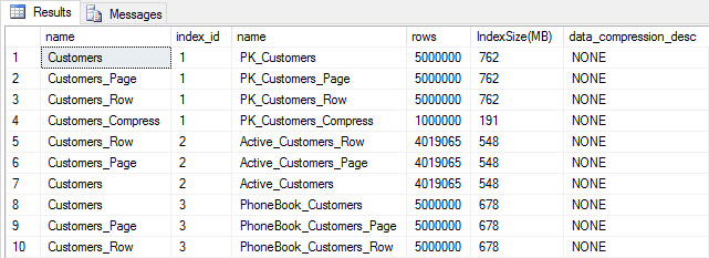 Table and index size after insert
As expected, all tables except Customers_Compress are about the same size. Now we'll rebuild indexes on all tables, implementing row and page compression on Customers_Row and Customers_Page, respectively.
ALTER INDEX ALL ON dbo.Customers REBUILD;
GO
ALTER INDEX ALL ON dbo.Customers_Page REBUILD WITH (DATA_COMPRESSION = PAGE);
GO
ALTER INDEX ALL ON dbo.Customers_Row REBUILD WITH (DATA_COMPRESSION = ROW);
GO
ALTER INDEX ALL ON dbo.Customers_Compress REBUILD;
If we check table size after compression, now we can see our disk space savings:
SELECT [o].[name], [i].[index_id], [i].[name], [p].[rows],
(8*SUM([au].[used_pages]))/1024 AS [IndexSize(MB)], [p].[data_compression_desc]
FROM [sys].[allocation_units] [au]
JOIN [sys].[partitions] [p]
	ON [au].[container_id] = [p].[partition_id]
JOIN [sys].[objects] [o]
	ON [p].[object_id] = [o].[object_id]
JOIN [sys].[indexes] [i]
	ON [p].[object_id] = [i].[object_id] AND [p].[index_id] = [i].[index_id]
WHERE [o].[is_ms_shipped] = 0
GROUP BY [o].[name], [i].[index_id], [i].[name], [p].[rows], [p].[data_compression_desc]
ORDER BY [i].[index_id], [IndexSize(MB)] DESC;
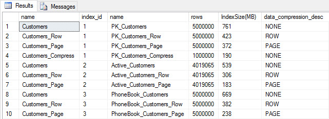
 Index size after compression
As expected, the row and page compression significantly decreases the size of the table and its indexes. The COMPRESS function saved us the most space – the clustered index is one quarter the size of the original table.
EXAMINING QUERY PERFORMANCE
Before we test query performance, note that we can use Query Store to look at INSERT and REBUILD performance:
SELECT [q].[query_id], [qt].[query_sql_text],
SUM([rs].[count_executions]) [ExecutionCount], AVG([rs].[avg_duration])/1000 [AvgDuration_ms],
AVG([rs].[avg_cpu_time]) [AvgCPU], AVG([rs].[avg_logical_io_reads]) [AvgLogicalReads],
AVG([rs].[avg_physical_io_reads]) [AvgPhysicalReads]
FROM [sys].[query_store_query] [q]
JOIN [sys].[query_store_query_text] [qt]
	ON [q].[query_text_id] = [qt].[query_text_id]
LEFT OUTER JOIN [sys].[objects] [o]
	ON [q].[object_id] = [o].[object_id]
JOIN [sys].[query_store_plan] [p]
	ON [q].[query_id] = [p].[query_id]
JOIN [sys].[query_store_runtime_stats] [rs]
	ON [p].[plan_id] = [rs].[plan_id]
WHERE [qt].[query_sql_text] LIKE '%INSERT%'
	OR [qt].[query_sql_text] LIKE '%ALTER%'
GROUP BY [q].[query_id], [q].[object_id], [o].[name], [qt].[query_sql_text], [rs].[plan_id]
ORDER BY [q].[query_id];
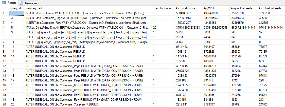 INSERT and REBUILD performance metrics
While this data is interesting, I'm more curious about how compression affects my everyday SELECT queries. I have a set of three stored procedures that each have one SELECT query, so that each index is used. I created these procedures for each table, and then wrote a script to pull values for first and last names to use for testing. Here is the script to create the procedures.
Once we have the stored procedures created, we can run the script below to call them. Kick this off and then wait a couple minutes…
SET NOCOUNT ON;
GO

DECLARE @RowNum INT = 1;
DECLARE @Round INT = 1;
DECLARE @ID INT = 1;
DECLARE @FN NVARCHAR(64);
DECLARE @LN NVARCHAR(64);
DECLARE @SQLstring NVARCHAR(MAX);

DROP TABLE IF EXISTS #FirstNames, #LastNames;

SELECT  DISTINCT [FirstName],
	DENSE_RANK() OVER (ORDER BY [FirstName]) AS RowNum
INTO #FirstNames
FROM [dbo].[Customers]

SELECT  DISTINCT [LastName],
	DENSE_RANK() OVER (ORDER BY [LastName]) AS RowNum
INTO #LastNames
FROM [dbo].[Customers]

WHILE 1=1
BEGIN
	SELECT @FN = (
		SELECT [FirstName]
		FROM #FirstNames
		WHERE RowNum = @RowNum)

	SELECT @LN = (
		SELECT [LastName]
		FROM #LastNames
		WHERE RowNum = @RowNum)

	SET @FN = SUBSTRING(@FN, 1, 5) + '%'

	SET @LN = SUBSTRING(@LN, 1, 5) + '%'

	EXEC [dbo].[usp_FindActiveCustomer_C] @FN;
	EXEC [dbo].[usp_FindAnyCustomer_C] @LN;
	EXEC [dbo].[usp_FindSpecificCustomer_C] @ID;
	EXEC [dbo].[usp_FindActiveCustomer_P] @FN;
	EXEC [dbo].[usp_FindAnyCustomer_P] @LN;
	EXEC [dbo].[usp_FindSpecificCustomer_P] @ID;
	EXEC [dbo].[usp_FindActiveCustomer_R] @FN;
	EXEC [dbo].[usp_FindAnyCustomer_R] @LN;
	EXEC [dbo].[usp_FindSpecificCustomer_R] @ID;
	EXEC [dbo].[usp_FindActiveCustomer_CS] @FN;
	EXEC [dbo].[usp_FindAnyCustomer_CS] @LN;
	EXEC [dbo].[usp_FindSpecificCustomer_CS] @ID;

	IF @ID < 5000000
	BEGIN
		SET @ID = @ID + @Round
	END
	ELSE
	BEGIN
		SET @ID = 2
	END

	IF @Round < 26
	BEGIN
		SET @Round = @Round + 1
	END
	ELSE
	BEGIN
		IF @RowNum < 2260
		BEGIN
			SET @RowNum = @RowNum + 1
			SET @Round = 1
		END
		ELSE
		BEGIN
			SET @RowNum = 1
			SET @Round = 1
		END
	END
END
GO
After a few minutes, peek at what's in Query Store:
SELECT [q].[query_id], [q].[object_id], [o].[name], [qt].[query_sql_text],
SUM([rs].[count_executions]) [ExecutionCount], CAST(AVG([rs].[avg_duration])/1000 AS DECIMAL(10,2)) [AvgDuration_ms],
CAST(AVG([rs].[avg_cpu_time]) AS DECIMAL(10,2)) [AvgCPU], CAST(AVG([rs].[avg_logical_io_reads]) AS DECIMAL(10,2)) [AvgLogicalReads],
CAST(AVG([rs].[avg_physical_io_reads]) AS DECIMAL(10,2)) [AvgPhysicalReads]
FROM [sys].[query_store_query] [q]
JOIN [sys].[query_store_query_text] [qt]
	ON [q].[query_text_id] = [qt].[query_text_id]
JOIN [sys].[objects] [o]
	ON [q].[object_id] = [o].[object_id]
JOIN [sys].[query_store_plan] [p]
	ON [q].[query_id] = [p].[query_id]
JOIN [sys].[query_store_runtime_stats] [rs]
	ON [p].[plan_id] = [rs].[plan_id]
WHERE [q].[object_id] <> 0
GROUP BY [q].[query_id], [q].[object_id], [o].[name], [qt].[query_sql_text], [rs].[plan_id]
ORDER BY [o].[name];
You'll see that most stored procedures have executed only 20 times because two procedures against [dbo].[Customers_Compress] are really slow. This is not a surprise; neither [FirstName] nor [LastName] is indexed, so any query will have to scan the table. I don't want those two queries to slow down my testing, so I'm going to modify the workload and comment out EXEC [dbo].[usp_FindActiveCustomer_CS] and EXEC [dbo].[usp_FindAnyCustomer_CS] and then start it again. This time, I'll let it run for about 10 minutes, and when I look at the Query Store output again, now I have some good data. Raw numbers are below, with the manager-favorite graphs below.
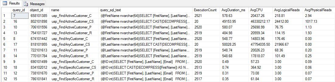 Performance data from Query Store
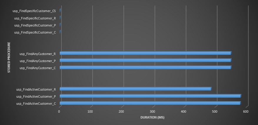 Stored procedure duration
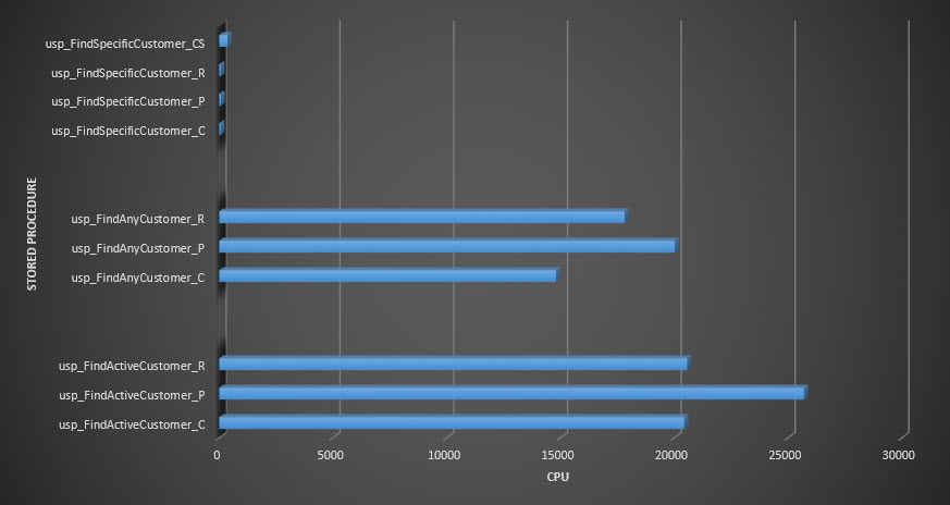 Stored procedure CPU
Reminder: All stored procedures that end with _C are from the non-compressed table. The procedures ending with _R are the row compressed table, those ending with _P are page compressed, and the one with _CS uses the COMPRESS function (I removed the results for said table for usp_FindAnyCustomer_CS and usp_FindActiveCustomer_CS as they skewed the graph so much we lost the differences in the rest of the data). The usp_FindAnyCustomer_* and usp_FindActiveCustomer_* procedures used nonclustered indexes and returned thousands of rows for each execution.
I expected duration to be higher for the usp_FindAnyCustomer_* and usp_FindActiveCustomer_* procedures against row and page compressed tables, compared to the non-compressed table, because of the overhead of decompressing the data. The Query Store data does not support my expectation – the duration for those two stored procedures is roughly the same (or less in one case!) across those three tables. The logical IO for the queries was nearly the same across the non-compressed and page and row compressed tables.
In terms of CPU, in the usp_FindActiveCustomer and usp_FindAnyCustomer stored procedures it was always higher for the compressed tables. CPU was comparable for the usp_FindSpecificCustomer procedure, which was always a singleton lookup against the clustered index. Note the high CPU (but relatively low duration) for the usp_FindSpecificCustomer procedure against the [dbo].[Customer_Compress] table, which required the DECOMPRESS function to display data in readable format.
SUMMARY
The additional CPU required to retrieve compressed data exists and can be measured using Query Store or traditional baselining methods. Based on this initial testing, CPU is comparable for singleton lookups, but increases with more data. I wanted to force SQL Server to decompress more than just 10 pages – I wanted 100 at least. I executed variations of this script, where tens of thousands of rows were returned, and findings were consistent with what you see here. My expectation is that to see significant differences in duration due to the time to decompress the data, queries would need to return hundreds of thousands, or millions of rows. If you're in an OLTP system, you don't want to return that many rows, so the tests here should give you an idea of how compression may affect performance. If you're in a data warehouse, then you will probably see higher duration along with the higher CPU when returning large data sets. While the COMPRESS function provides significant space savings compared to page and row compression, the performance hit in terms of CPU, and the inability to index the compressed columns due to their data type, make it viable only for large volumes of data that will not be searched.
The post Compression and its Effects on Performance appeared first on SQLPerformance.com.
26 Jan 07:32

Year-over-year comparison using the same number of days in #dax
by Marco Russo (SQLBI)
When you use the time intelligence functions in DAX, it is relatively easy to filter the same dates selection in the previous year by using the SAMEPERIODLASTYEAR or DATEADD functions. However, if you follow the best practices, it is likely that you have a full date table for the current year, which includes many days in the future. If you are in the middle of March 2017, you have sales data until March 15, 2017, so you might want to compare such a month with the same number of days in 2016. And the same when you compare the Q1, or the entire year.
A common solution is to translate this request in a month-to-date (MTD) or quarter-to-date (QTD) comparison, but depending on how you implement this, you might not obtain a reliable result. For example, you might assume that the current date on your PC is the boundary of the dates you want to consider, but you probably have a few hours if not days of latency in the data in your database, so you should constantly fix the offset between the current day and the last day available in your data.
Thus, why not simply relying on the data you have to make an automatic decision? This is the purpose of the technique described in the article Compare equivalent periods in DAX that I wrote on SQLBI, where I show several approaches optimized for Power BI, Excel, and SSAS Tabular, which are different depending on the version you use.
Personally, the version I prefer is the one with the variables in DAX:
[PY Last Day Selection] :=

VAR LastDaySelection =

    LASTNONBLANK ( 'Date'[Date], [Sales Amount] )

VAR CurrentRange =

    DATESBETWEEN ( 'Date'[Date], MIN ( 'Date'[Date] ), LastDaySelection )

VAR PreviousRange =

    SAMEPERIODLASTYEAR ( CurrentRange )
    RETURN
    IF (

        LastDaySelection > MIN ( 'Date'[Date] ),

        CALCULATE ( [Sales Amount], PreviousRange )

    )
     It’s longer, but much more readable. More details and examples you can download for Excel and Power BI are available in the article.
26 Jan 07:32
December 2016 Leaderboard of Database Systems contributors on MSDN
by SQL Server Team
This post was authored by Rahul Venkatraj, Program Manager, Data Platform Group
We continue to receive encouraging comments from the community on the Leaderboard. Thank you.
Many congratulations to the top-10 contributors featured on our December leaderboard!

Olaf Helper and Alberto Morillo top the Overall and Cloud database this month. Six of this month’s Overall Top-10 (including all of the top three) featured in last month’s Overall Top-10 as well, and four others are new entrants.
The following continues to be the points hierarchy (in decreasing order of points):

For questions related to this leaderboard, please write to leaderboard-sql@microsoft.com.
26 Jan 07:31
SQL Server named DBMS of the Year by DB-Engines
by SQL Server Team
SQL Server was recently named DBMS of the Year by DB-Engines. DB-Engines is an initiative to collect and present information on database management systems, and provides a widely accepted popularity ranking of database management systems, and has been created and maintained by solid IT, an Austrian company with a special focus on database consulting and software development. In their award announcement recognizing SQL Server as the DBMS gaining the most popularity in 2016, DB-Engines cites the “release of SQL Server 2016 and the announcement to port SQL Server to Linux” and also highlights SQL Server’s strength in their ranking categories of job offers, LinkedIn profiles, and other ranking components.
We strive to deliver choice to our customers and to continually empower them to do more. SQL Server 2016 enables industry-leading performance and security [1] with built-in business intelligence on any device, as well as in-database advanced analytics, at industry-leading TCO. In 2016, we also made our fully-featured SQL Server Developer Edition free for development and testing. [2] With SQL Server 2016 Service Pack 1, we have made key innovations more accessible to developers and organizations across SQL Server editions, making it easier than ever to build advanced applications that scale across editions. Finally, the next release of SQL Server, currently in public preview, brings even more choice to developers, with the abilities to run SQL Server on Linux, Docker Engine, macOS on Docker for Mac, in addition to Windows.
Thank you to DB-Engines for this award, and to our customers for your continued support. We are grateful to have such a passionate user community. Please feel free to share your input about SQL Server using Microsoft’s Connect tool.
For those who haven’t used SQL Server 2016 or SQL Server v.Next yet, here are a few resources to learn more:
- Keep up with the latest news and information on the SQL Server webpage
- Get started today with public preview of next version of SQL Server on Linux or Windows
- Download SQL Server Developer Edition and our developer tools and build an app using SQL Server
[1] National Institute of Standards and Technology Comprehensive Vulnerability Database, 2016.
[2] Development and testing only; not for production or use with production data
26 Jan 07:31

Hack-Attaching a SQL Server database with NORECOVERY
by Argenis
Let me just start this post with a huge disclaimer/warning: what I'm about to show you in this post is NOT SUPPORTED by Microsoft at all. It's a hack, and it might not work whatsoever in your environment.
But I think it's pretty cool.
You might have probably heard about hack-attaching a database. It's a very good thing to know, and a powerful tool when you need it. That's not supported by Microsoft either (technically speaking), but I've seen folks use it. I may or may not have used it more than once :)
Whenever you attach a database to SQL Server, crash recovery is executed against it - and it is always brought online automatically. Requests from the community - and vendors, even - to Microsoft to implement a means to attach a database with NORECOVERY (such that you can later apply transaction log backups to it) have gone nowhere - closed as "Won't fix" in Connect. Some folks have blogged on their approach to how to do this, but I have found myself with mostly suspect or plain unusable databases while trying them.
In this post I will detail the steps that worked for me to make this possible - and even initializing an AlwaysOn Availability Groups replica leveraging a hack-attached database with NORECOVERY.
In a Pure Storage-hosted post I used StackOverflow's publicly-accessible database to discuss dedupe and compression in our arrays - in this post I use that database again.
To get started, I logged on to CSLAB-SQL00, and I took a VSS snapshot of the volume where the data and log files for this database live. Please note that you don't really need VSS for certain storage arrays, like Pure Storage FlashArrays, which always generates crash-consistent snaps and copies. Since a Pure Storage array is all I have access to, this is what I will use for the purposes of this blog post, but I wanted to use VSS to keep the process generic and applicable to other storage arrays.

Please note that the failed COM call shown above can be safely ignored, per this Microsoft KB article.
Using the FlashArray GUI, I create a volume from the snapshot:
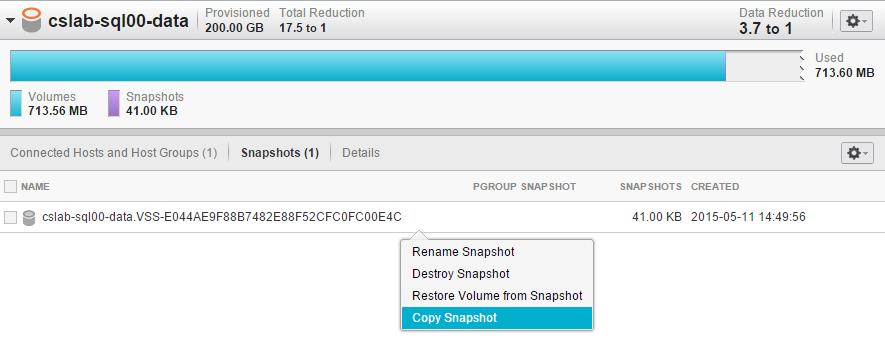
The GUI asks for a name for the new volume, so I picked one:
Now let's present the new volume to CSLAB-SQL01, a different server attached to the same array. In this case I could also leverage the array's replication capabilities to have a snapshot, possibly of a protection group if your data and log files live on a separate volume, replicated to another array.
Presenting a volume to a host using the GUI couldn't be easier. Click on the gear icon, choose Connect Hosts and select the host you want. Then click Confirm, and off you go.
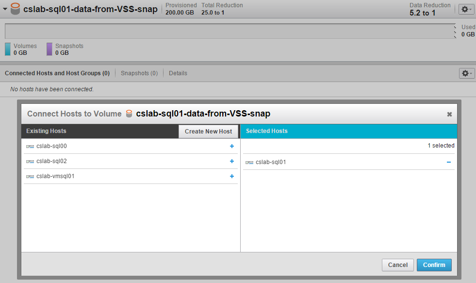
I now log on to CSLAB-SQL01, and issue a Rescan Disks on Disk Management. Keep in mind that all of this could be scripted using Pure's Powershell SDK. This guy pops up on the list:

And now I use some DISKPART goodness to bring the volume online, and with a new disk signature, which is needed here only because CSLAB-SQL00 and CSLAB-SQL01 are nodes of the same Windows Server Failover Cluster (WSFC), and clear out some attributes:

If you're wondering where I got that GUID from, I executed [GUID]::NewGuid() on another Powershell window. You could also execute SELECT NEWID() on any SQL Server instance to get a new GUID.
I mounted the new volume on X:\SqlData2 then granted NT SERVICE\MSSQLSERVER full control on the files.
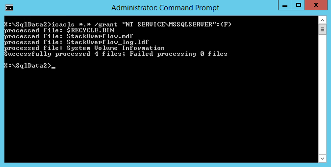
To confirm that SQL Server can access the files, I issued a convenient DBCC CHECKPRIMARYFILE:
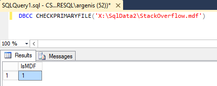
Much like in the traditional hack-attach approach, we create an empty database on the target instance. This is going to be on the X:\SqlData mount point/volume. You will need to make sure that file names and database file IDs match, otherwise you might not get things to work.
If you have Instant File Initialization (IFI) enabled, and you use a FlashArray volume to host this empty database, it will take very little space -- and it will only take a few seconds to create. In my test machine, this took about 650Kb of actual disk space and less than 2 seconds to complete.
I then took a full backup of the empty database (to FILE='nul', of course) and a tail of the log backup, to bring the empty database to Restoring status:

Now, we stop SQL Server and replace the volume mounted on X:\SqlData with the one that was mounted on X:\SqlData2, and start SQL Server again.
If you try to bring the database to STANDBY/Read-only, you should get something similar to this:
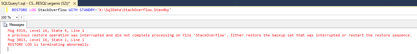
But CONTINUE_AFTER_ERROR comes to the rescue:
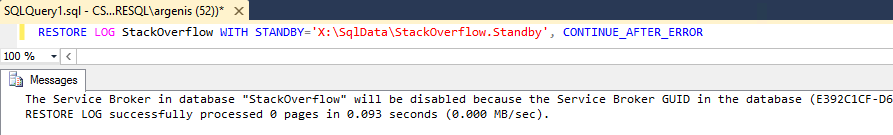
Now pay attention to the message that got cropped on my screenshot above: if you use Service Broker with your original database, you will have to enable it later.
We now have a database in STANDBY. Could we possibly restore some transaction log backups on top of it? You bet! I went to the source database, and created a dummy table with 1000 rows, then took a transaction log backup:
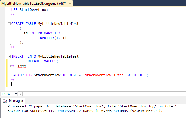
I copied the transaction log backup file to the target host (CSLAB-SQL01). This is what I got when I tried to restore it -- same error as when I put the database in STANDBY, basically:

Yep, CONTINUE_AFTER_ERROR to the rescue, again:

The database is now in NORECOVERY! To confirm I have a good database, I put the database in STANDBY again, then proceed to query the dummy table:

1000 rows there, so it looks like all is well. But is my database COMPLETELY clean?
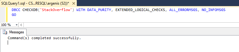
A clean CHECKDB -- music to my ears.
Now you might be wondering: can I use this hack-attached database with NORECOVERY to join this database to an availability group? Yes. Can I make it a mirroring partner? Yup! How about a log shipping secondary? That too. Can this help you in case of "Oops, I dropped a table in production!"? You bet.
Some of you be thinking "Hey, can't I just use a VSS requester app like Commvault, Netbackup or Catalogic to do this?" Of course you can. This post is targeting those of you who don't have that choice.
To recap: I went from a SAN snapshot to point-in-time recovery in a couple minutes. I think that's pretty cool. But remember, this stuff isn't supported!
Thanks for reading,
-A
26 Jan 07:31
The Recording for Advanced SSIS Execution is Available
by andyleonard
The recording for the Enterprise Data & Analytics webinar titled Advanced SSIS Execution is now available (registration required). Enjoy! :{> Learn More: SSIS Catalog Compare v2.0 Launch Event 7 Mar 2017! SSIS Catalog Management SSIS Lifecycle...(read more)
26 Jan 07:31
Debugging Complex SQL Queries
by Michael Blaha
We favor the offloading of application logic to SQL queries. Developers can save time, effort, and reduce mistakes by substituting SQL for programming code. This leads to lengthy and complex SQL that must be debugged. It is common to write a SQL query that initially fails to execute. By misspelling a name. By omitting a […]
The post Debugging Complex SQL Queries appeared first on DATAVERSITY.
18 Jan 21:22
NICE Introduces Nexidia Analytics – the Next Generation of Interaction Analytics
by A.R. Guess
by Angela Guess According to a new press release, “NICE introduces its next generation interaction analytics solution, based on the Nexidia platform, which sets a new standard for accurate, real-time omni-channel analysis. The Nexidia Analytics solution, which incorporates best-of-breed capabilities from both Nexidia and NICE, uses deep learning neural networks to perform sophisticated audio and […]
The post NICE Introduces Nexidia Analytics – the Next Generation of Interaction Analytics appeared first on DATAVERSITY.
18 Jan 21:09
Introducing astreams
by andyleonard
For months, I’ve received pings about a screenshot I posted on social media a year or so ago. Plus I needed to wind down. You real runners will know what I mean: You know how you feel after you’ve covered some distance (for you)? You need to walk around for a bit, you can’t just stop cold. You need to wind down. I needed that after the effort to release SSIS Catalog Compare v2. astreams became the coding-equivalent of a wind down. I’d been using another application that kind-of-sort-of did what astreams...(read more)
18 Jan 20:58


What’s New in SQL Server 2016 Reporting Services–Now live at Pluralsight
by arcanecode
So you want to see what’s new in SQL Server 2016 Reporting Services? Well I’ve got just the thing for you. My 12th course just went live on Pluralsight, named appropriately “What’s New in SQL Server 2016 Reporting Services”.
This course is designed specifically for those who are already familiar with SQL Server Reporting Services, and just need to come up to speed with the new features in the 2016 release. Even better you can do it during a long lunch (or two short ones), the course is just under an hour and a half so you can learn quickly.
The course starts with a look at the brand new Report Portal, the replacement for Report Manager. You’ll see how to create KPIs right in the portal, improvements to subscriptions, and how to custom brand the Report Portal so it can integrate right into your companies websites. After that you’ll learn about the new HTML 5 compatibility, something that makes SSRS integrate even better into your web apps and sites.
Some time is then spent on improvements to what Microsoft calls “Paginated Reports”, essentially the same reports you’ve grown to know and love. You’ll see improvements for embedded reports, as well as the two new chart types, sunburst and treemap. Finally, the long awaited ability to arrange parameters is covered.
Last, but certainly not least, the course covers what I consider to be the most exciting piece of the 2016 release, the Mobile Report Publisher. You’ll see how to use it to generate reports, and how they can be used on the web as well as mobile devices such as phones and tablets.
What’s that you say? You want to see it, but don’t have a Pluralsight subscription? Hey, no problem. Just shoot me an email, free at arcanetc.com. I can send you a code good for 30 days during which you can watch this and any of the over 5,000 (yes, FIVE THOUSAND) courses.
18 Jan 20:56

VertiPaq Analyzer 1.7: a fundamental tool for #powerbi #powerpivot #ssas #tabular diagnostics and documentation
by Marco Russo (SQLBI)
If you work with Power Pivot, Power BI, or Analysis Services Tabular, you probably already know VertiPaq Analyzer. If you never used it, with the new release 1.7 you have another couple of very good reason to try it.
VertiPaq Analyzer is a Power Pivot workbook that extracts information from data management views (DMVs) of a Tabular model. It can be connected to a SSAS Tabular or a Power BI database. If you have a Power Pivot data model, just import it in Power BI and extracts the information from there. You will quickly see what are the tables and columns that are more expensive, and you will have all the details about cardinality of columns and tables at a glance. This is of paramount importance when you have to optimize a DAX expression. However, these are the features we already had in VertiPaq Analyzer. What’s new in this release?
- There are two versions of the VertiPaq Analyzer, which is an Excel file with VBA macros now (for the new VertiPaq Analyzer ribbon)
- The version with suffix 1103 uses the “legacy” DMVs for Multidimensional
- The version with suffix 1200 starts using the new DMVs for Tabular (which are available only for compatibility level 1200 – more on that in this article.
- There is a ribbon for VertiPaq Analyzer that includes a button to format all the DAX expressions:

- And yes, there are three new worksheets that show all the measures, calculated columns, and calculated tables extracted from the data model, each one with its own DAX expression
- Last but not least, the Relationships worksheet shows in a clear way the tables and columns involved for each relationship, including two measures about the maximum cardinality of the columns involved in the relationship.

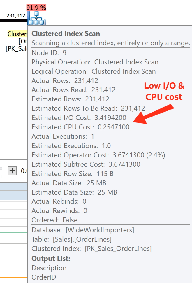
This tool is amazing to do remote troubleshooting, or even just to document what are the DAX formulas you have in a model at a given point in time. It saves me hours every week. I hope it will be useful to you, too!
18 Jan 20:52
NI Debuts Industrial Internet of Things (IoT) Lab to Promote Innovation and Collaboration
by A.R. Guess
by Angela Guess A new press release reports, “NI, the provider of solutions that enable engineers and scientists to solve the world’s greatest engineering challenges, announced today the opening of the new NI Industrial IoT Lab at its Austin headquarters. The NI Industrial IoT Lab focuses on intelligent systems that connect operational technology, information technology […]
The post NI Debuts Industrial Internet of Things (IoT) Lab to Promote Innovation and Collaboration appeared first on DATAVERSITY.
18 Jan 20:52
A Comparative Study of Business Intelligence and Analytics Market Trends
by Paramita Ghosh
The global Business Intelligence and Analytics market this year has already reached or is nearing $16.9 Billion, according to Gartner. The BI and Analytics market has undergone a major transformation from an enterprise IT-led, record reporting system to business-driven self-service data explorations. This turnaround of trends in Business Intelligence (BI) and Analytics indicates a larger […]
The post A Comparative Study of Business Intelligence and Analytics Market Trends appeared first on DATAVERSITY.
18 Jan 20:49

Automating DBCC PAGE, part 2 – determining object names on pages
by Wayne Sheffield
In a prior blog post, I demonstrated how using DBCC PAGE can be automated by using the “WITH TABLERESULTS” option. In this post, we will continue with another look at how this can be done.
On a nice wintry day, your city ended up being covered in several feet of snow. During the course of the night, your own house had several power outages. Being concerned about your databases, you shoveled your way into your office, so that you could check on things. (Okay… actually you would just VPN in, but this is my story after all…)
Once you get into your server, you check the jobs and find that your job that runs DBCC CHECKDB has failed. Let’s assume that a power glitch has caused corruption in your database. In order to find out what all is affected, you run DBCC CHECKDB WITH NO_INFOMSGS, ALL_ERRORMSGS. But, this happens to be on your 2TB database, and it will take a while for CHECKDB to finish so that you can find the scope of corruption.
You’d really like to know what tables are affected without having to wait. Luckily(?), this corruption was recorded in msdb.dbo.suspect_pages, and having just recently read Paul Randal’s post here, we know we can use DBCC PAGE to determine this information. And, after having read my prior blog post, you know that we can automate DBCC PAGE, so we can use our new friend “WITH TABLERESULTS” to find out what objects have been corrupted.
The suspect_pages table, documented here, has three particular columns of interest: database_id, file_id and page_id. These correspond nicely to the first three parameters needed for DBCC PAGE. To automate this, we need to know what information we need to return off of the page – and from Paul’s post, we know that this is the field “METADATA: ObjectId”. For this code example, let’s assume that this corruption is on page 11 of the master database (just change “master” to the name of your 2TB database).
IF OBJECT_ID('tempdb.dbo.#DBCCPAGE') IS NOT NULL DROP TABLE #DBCCPAGE;
CREATE TABLE #DBCCPAGE (
       ParentObject VARCHAR(255),
       [Object]     VARCHAR(255),
       Field       VARCHAR(255),
       [VALUE]     VARCHAR(255));
INSERT INTO #DBCCPAGE
EXECUTE ('DBCC PAGE (''master'', 1, 11, 3) WITH TABLERESULTS;');

SELECT schema_name = OBJECT_SCHEMA_NAME(ca.object_id),
       object_name = OBJECT_NAME(ca.object_id)
FROM   #DBCCPAGE
       CROSS APPLY (SELECT CONVERT(INTEGER, VALUE)) ca(object_id)
WHERE   Field = 'Metadata: ObjectId';
And there you go… you now know which object it is that has the corruption. In the same fashion, another interesting field that is returned is the IndexId – the Field value is “Metadata: IndexId”. It would be a similar exercise to grab that from this page also, an exercise that I’ll leave to you.
An automated method for getting the object from all suspect pages would entail encapsulating this logic into a cursor to spin through each row in the suspect_pages table (and I’ll even throw in getting the index_id also):
IF OBJECT_ID('tempdb.dbo.#DBCCPAGE') IS NOT NULL DROP TABLE #DBCCPAGE;
IF OBJECT_ID('tempdb.dbo.#SuspectObjects') IS NOT NULL DROP TABLE #SuspectObjects;
CREATE TABLE #DBCCPAGE (
        ParentObject    VARCHAR(255),
        [Object]        VARCHAR(255),
        Field           VARCHAR(255),
        [VALUE]         VARCHAR(255));
CREATE TABLE #SuspectObjects (
        database_id     INTEGER,
        file_id         INTEGER,
        page_id         INTEGER,
        object_id       INTEGER,
        index_id        INTEGER);
DECLARE @database_id    INTEGER,
        @file_id        INTEGER,
        @page_id        INTEGER,
        @SQLCMD         NVARCHAR(MAX);

DECLARE cCrackSuspectPages CURSOR LOCAL FAST_FORWARD FOR
SELECT  'EXECUTE (''DBCC PAGE (' +
            CONVERT(VARCHAR(15), database_id) + ', ' +
            CONVERT(VARCHAR(15), file_id) + ', ' +
            CONVERT(VARCHAR(15), page_id) + ') WITH TABLERESULTS;'');',
        database_id, file_id, page_id
FROM    msdb.dbo.suspect_pages;

OPEN cCrackSuspectPages;
FETCH NEXT FROM cCrackSuspectPages INTO @SQLCMD, @database_id, @file_id, @page_id;
WHILE @@FETCH_STATUS = 0
BEGIN
    TRUNCATE TABLE #DBCCPAGE;
    INSERT INTO #DBCCPAGE EXECUTE (@SQLCMD);

    INSERT INTO #SuspectObjects
            (database_id,
             file_id,
             page_id,
             object_id,
             index_id
            )
    SELECT  @database_id, @file_id, @page_id,
            (SELECT CONVERT(INTEGER, VALUE)
             FROM   #DBCCPAGE dp
             WHERE  dp.Field = 'Metadata: ObjectId'),
            (SELECT CONVERT(INTEGER, VALUE)
             FROM   #DBCCPAGE dp
             WHERE  dp.Field = 'Metadata: IndexId');

    FETCH NEXT FROM cCrackSuspectPages INTO @SQLCMD, @database_id, @file_id, @page_id;
END
CLOSE cCrackSuspectPages;
DEALLOCATE cCrackSuspectPages;

SELECT  database_name = DB_NAME(database_id),
        database_id,
        file_id,
        page_id,
        schema_name = OBJECT_SCHEMA_NAME(object_id, database_id),
        object_name = OBJECT_NAME(object_id, database_id),
        index_id
FROM    #SuspectObjects;
If you happen to be on SQL 2012 or higher, this can be greatly simplified by using the new (undocumented) DMO function sys.dm_db_database_page_allocations (and it also takes away the need to crack the page using DBCC PAGE).
SELECT  database_name = DB_NAME(sp.database_id),
        sp.database_id,
        sp.file_id,
        sp.page_id,
        schema_name = OBJECT_SCHEMA_NAME(dpa.object_id, sp.database_id),
        object_name = OBJECT_NAME(dpa.object_id, sp.database_id),
        dpa.index_id
FROM    msdb.dbo.suspect_pages sp
CROSS APPLY sys.dm_db_database_page_allocations(sp.database_id, NULL, NULL, NULL, 'LIMITED') dpa
WHERE   sp.file_id = dpa.allocated_page_file_id
AND     sp.page_id = dpa.allocated_page_page_id;
And there we go – yet another time when you might want to automate using DBCC PAGE. By now you should be able to see other uses for it – as long as you can get the database_id, file_id and page_id, you can automate the usage of it to retrieve the information that you are looking for.
Previous related posts:
Persisting DBCC Output
Automating DBCC Page
This post is re-published from my original post on SQL Solutions Group.
The post Automating DBCC PAGE, part 2 – determining object names on pages appeared first on Wayne Sheffield.