bis zu 6°CProistosescu & Huybers 2017
Pressemitteilung hier; ein wirklich heftiges Alarmpaper, das es wohl darauf anlegt, im 6. IPCC-Bericht zitiert zu werden und den Mittelwert aller Studien nach oben zu ziehen. Nic Lewis hat das Ganze detailliert auf Climate Audit auseinandergenommen.
3,7°C Brown & Caldeira 2017
Auch dies wohl eher ein Ausreißer nach oben. Das gibt kräftig Fördergelder.
1,3°CSpencer 2018
Szenario, dass nur 70% der Erwärmung der letzten 150 Jahre anthropogenen Ursprungs sind. Die mögliche Klimawirkung der Sonne ist in den meisten Berechnungen der Klimasensitivität gar nicht enthalten.
Zum Vergleich: In unserem Buch ‘Die kalte Sonne’ stellten wir ein 1,5°C-Szenario dar. Das liegt am unteren Ende der Spannbreite des IPCC AR5-Berichts, 1,5-4,5°C.
Zum Vergleich: Der TCR Durchschnitt aller Klimamodelle im IPCC AR5-Bericht betrug 2.31 °C.
Alles deutet auf eine seismische Verschiebung im Verständnis der CO2-Klimasensitivität im gerade entstehenden 6. IPCC-Bericht hin. Der ‘beste Schätzwert’ wird sich auf jeden Fall deutlich nach unten bewegen. Das bereitet eingefleischten Klimakämpfern natürlich bereits jetzt schon Bauchschmerzen. Sie bereiten die Welt bereits auf die Veränderungen behutsam vor. So schrieben Knutti et al. 2017 in Nature Geoscience, dass man auf jeden Fall die Treibhausgasemissionen weiter einschränken müsse, egal ob der Wert der CO2-Klimasensitivität nun möglicherweise niedriger liegt:
Jenseits der Gleichgewichts-Klimasensitivität ECS
Die Gleichgewichts-Klimasensitivität charakterisiert die langzeitliche Reaktion der globalen Temperatur auf eine gestiegene atmosphärische CO2-Konzentration. Sie hat als Einzelzahl fast den Status einer Ikone erreicht als Maßzahl, wie ernst die Klimaänderung sein wird. Der Konsens der „wahrscheinlichen“ Bandbreite der Klimasensitivität von 1,5°C bis 4,5°C von heute ist die Gleiche, welche Jule Charney schon im Jahre 1979 genannt hatte, doch basiert sie heute auf quantitativen Beweisen aus dem gesamten Klimasystem und über die gesamte Klima-Historie. Der Kreuzzug bzgl. der Klimasensitivität hat bedeutende Einsichten in die Zeitmaßstäbe der Reaktion des Klimasystems vermittelt, der natürlichen Variabilität und Grenzen von Beobachtungen und Klimamodellen. Aber es ergaben sich auch Bedenken hinsichtlich der einfachen Konzepte, welche der Klimasensitivität und dem Strahlungsantrieb zugrunde liegen. Dies wiederum ebnet den Weg zu einem besseren Verständnis der Klima-Reaktion auf Antriebe. Schätzungen der Transient Climate Response TCR sind eher abhängig von der beobachteten Erwärmung und sind relevanter für die Prognose der Erwärmung während der kommenden Jahrzehnte. Neuere Verknüpfungen, welche globale Erwärmung in direkte Relation zum insgesamt emittierten CO2 setzen zeigen, dass wenn man die Erwärmung unter 2°C halten will man die zukünftigen CO2-Emissionen stark limitieren muss, unabhängig davon, ob die Klimasensitivität hoch oder niedrig ist.
Dabei verschleiern die Autoren, dass Werte am unteren Ende des Spektrums eine deutlich weniger dramatische Lage repräsentieren als die höheren Werte, die uns vielleicht wirklich in eine Klimakatastrophe gestürzt hätten. Die Zeit der Rechtfertigungen hat begonnen, “wir haben es ja nur gut mit Euch gemeint”. Ebenfalls erst vor ein paar Monaten mussten Millar et al. 2017 einräumen, dass die Klimamodelle wohl in der Tat viel zu heiß laufen und das 1,5-Gradziel auch mit der dreifachen Menge an CO2-Emissionen erreicht werden kann.
Andere wollen die neuen Realitäten immer noch nicht wahr haben. Ein Team um Kate Marvel (darunter auch der bekennende Klimaaktivist Gavin Schmidt) behauptete im Februar 2018 in den Geophysical Research Letters, dass die reale Temperaturentwicklung der letzten Jahrzehnte gar nicht dazu taugt, die CO2-Klimasensitivität zu berechnen. Korrekt wären vielmehr die theoretischen Simulationen aus dem Computer. Das hinterlässt einen schon ziemlich sprachlos. Nic Lewis analysierte das Paper und entdeckte eine Vielzahl von Problemen. Die Vorphase zum 6. IPCC-Bericht treibt wundersame Blüten. Beide Seiten laufen zu Höchstleistungen auf, um ihre Sichtweise zitierbar zu dokumentieren. Da scheinen auch die absurdesten Publikationen jetzt durchzukommen, wenn Gutachter mit ähnlicher Gesinnung gefunden werden können.
Fahrverbote sind also zulässig. Das sagt das Bundesverwaltungsgericht in Leipzig. Städte können grundsätzlich Fahrverbote für Dieselautos verhängen. Das sei vom geltenden Recht gedeckt. Eine bundesweite Regelung sei dafür nicht notwendig.
Der schwarze Peter liegt bei den Städten
Damit sind die beiden Länder Baden-Württemberg und Nordrhein-Westfalen mit ihrer Revision gescheitert. In Düsseldorf und Stuttgart hatte die dubiose Abmahnorganisation Deutsche Umwelthilfe (DUH) geklagt, weil die Städte die neuen herabgesetzten EU-Grenzwerte nicht einhalten würden. Im Zweifel, daraufhin klagte die DUH, sollten die Städte ihre Straßen für Autos sperren. Damit liegt der Schwarze Peter bei den Städten – sie sollen die Autofahrer schröpfen und enteignen, um unrealistische Grenzwert auf Teufel komm raus einzuhalten.
Denn grundsätzlich seien solche Fahrverbote durch das Recht gedeckt, meinte jetzt das Bundesverwaltungsgericht. Damit öffnet das Gericht ein weiteres schönes Betätigungsfeld für Angehörige des Justizwesens. Geprüft werden muss laut Leipziger Entscheidung, ob bei einem Fahrverbot die Verhältnismäßigkeit gewahrt bleibt. Was auch immer das im Einzelfall heißt – es dürfte jetzt Gegenstand von vielen munteren Klagen werden. Denn Fahrverbote müssen immer Einzelfallentscheidungen sein, gegen wiederum juristisch vorgegangen werden kann.
Von der Umwelt- zur Rechtsanwaltshilfe
Ein Mittel könnte eine Klage auf flüssigere Verkehrsführung sein. Weniger Staus – das bedeutet auch weniger Luftbelastung, wie gerade Stuttgart an einigen Straßen belegt hat. Was immer sie tun – die Städte riskieren teure Prozesse. Aus der Umwelthilfe wird eine Art Rechtsanwaltshilfe.
Klagen könnten auch Autobesitzer gegen Hersteller, um ihren alten Dieselwagen loszuwerden, den Hersteller in Anspruch zu nehmen und Wagen zurückzunehmen.
Wobei „alt“ bereits bei zwei bis vier Jahren losgehen kann. Früher war das noch kein Alter für ein Auto, heute kann es Schrottwert bedeuten. Immerhin mussten Dieselbesitzer rund 15 bis 20 Prozent Wertverluste hinnehmen in den letzten Jahren.
Jetzt nach dem Leipziger Urteilsspruch vermutlich noch mehr. Bis zu 15 Milliarden Euro könnte ein Fahrverbot für Dieselfahrzeuge kosten, hat der Professor für Automobilwirtschaft Ferdinand Dudenhöffer ausgerechnet.
Kosten, deren Verantwortliche klar benannt werden können.
Die Reaktionen fielen sehr unterschiedlich aus. Für Christian Lindner (FDP) ein „Schlag gegen Freiheit und Eigentum, weil wir uns zu Gefangenen menschengemachter Grenzwerte machen“. Er will in Zukunft Grenzwerte auf Basis solider wissenschaftlicher Debatte.
Die geschäftsführende Umweltministerin Hendricks sieht die Autohersteller in der Pflicht zur Nachrüstung, also sozigerechter Aktionismus, gutes Geld schlechtem hinterherzuwerfen, ohne dass ein Nutzen herauskommt.
Bundesregierung und Parteien spielen den Unschuldigen
Windelweich die Reaktion der Nichtregierung in Berlin. Die CDU/CSU-Bundestagsfraktion schreibt: „Kommunen können demnach selbst entscheiden, ob sie an bestimmten Stellen eingreifen. Eine Regelung des Bundes ist dafür nicht notwendig, also auch keine blaue Plakette. Ausdrücklich weist das Gericht auch darauf hin, dass bei den Luftreinhalteplänen die Verhältnismäßigkeit gewahrt werden muss. Unser Ziel bleibt es, auch künftig die innerstädtische Luftqualität weiter zu …“
Das sind flotte Sprüche, die den Betroffenen nicht helfen – nicht den Städten, den Bürgern und schon gar nicht den Autofahrern. Dabei wird die klagende Deutsche Umwelthilfe massiv mit Bundesmitteln unterstützt. Wenn sich jetzt die Bundesregierung versucht wegzuducken, dann ist das nicht glaubhaft glaubhaft. Es war die Bundesregierung, die für die Grenzwerte wie für das Vorgehen der DUH die Verantwortung trägt – und jetzt so tut, als habe sie damit nichts zu tun.
Der lange Weg des Irrsinns
Die Entwicklung des Irrsinns deutete sich seit langem an. Die politischen Grundlagen sind von rot-grünen Stoßtrupps schon in den 90er Jahren gelegt worden. Damals empfahl die grün dominierte Weltgesundheitsorganisation WHO 40 Mikrogramm pro Kubikmeter Stickoxide. Noch nicht einmal Kalifornien als Umweltvorreiter hatte einen solchen Grenzwert festgelegt. In den USA gelten heute 100 Mikrogramm pro Kubikmeter. Die EU jedenfalls wählte 1999 40 Mikrogramm pro Kubikmeter als künftigen Grenzwert.
Vor etwa zehn Jahren wurden heutigen Abgasgrenzwerte für Autos festgelegt, also die Emissionswerte. Die Ingenieure wussten seinerzeit nicht, wie sie die überhaupt erreichen könnten. Es gab noch keinerlei Technologien dafür.
„Ein Wert, der mit der Dartscheibe geworfen wurde“, sagt heute Werner Ressing, ehemaliger Ministerialdirektor im Bundeswirtschaftsministerium, der damals die Verhandlungen in Brüssel für Deutschland führte. Er, der sich mit am längsten mit den Grenzwerten beschäftigt hat, stellte jetzt auch in seiner Stellungnahme für das Bundesverwaltungsgericht klar:
„Mir ist klar, dass die 40 Mikrogramm NO2 der geltende Grenzwert sind: Gleichwohl möchte ich als früher zuständiger Beamter des BMWi Ihren Blick darauf lenken, dass dieser Grenzwert relativ willkürlich gewählt wurde und Sie als unabhängiges Gericht die Politik auffordern sollten, diesen Grenzwert zu ändern.“
Denn, so Ressing, der 40 Mikrogramm-Grenzwert wurde von der WHO nicht empfohlen, sondern von der EU aus einem Sammelsurium von WHO-Grenzwerten willkürlich festgelegt.
Medizinisch sei der Grenzwert nicht zu begründen. Zudem gelten völlig unterschiedliche Grenzwerte für zum Beispiel Büroarbeitsplätze von 60 µg/Kubikmeter, am Arbeitsplatz gelten als maximaler Wert 950 in der Schweiz sogar 6.000 Mikrogramm pro Kubikmeter.
Ressing verweist auf die USA: Dort gelten im Verkehr 100 Mikrogramm und es gibt keine Fahrverbote; 100 Mikrogramm werden in jeder deutschen Stadt unterschritten.
Ressings Fazit: „Der Grenzwert ist willkürlich gewählt und viel zu niedrig. Fahrverbote hätten unabsehbare wirtschaftliche Konsequenzen und sind deshalb unverhältnismäßig.“
Seine Aufforderung als Reaktion auf das Leipziger Urteil: Die Politik muss nach Brüssel marschieren und den Grenzwert ändern! Aber genau das verweigert bislang die Bundesregierung. Sie lässt Brüssel die Schmutzarbeit erledigen und hofft, dass sie trotzdem weiter Wählerstimmen kassiert, weil die Verantwortung doch in Brüssel liege. Aber genau das ist falsch – in Berlin sitzen die Verantwortlichen für das Elend von Millionen Autobesitzern, Handwerkern und Berufstätigen, die jetzt neue Autos kaufen sollen.
Mit Umweltschutz hat es nichts zu tun
Es gibt keinerlei Belege dafür, dass Stickoxide in den Straßen zu Erkrankungen führen – jedenfalls nicht in jenen geringen Konzentrationen, wie sie in bestimmten Bereichen der Innenstädte zu finden sind. Vollkommener Unsinn ist die Rede von 10.000 Toten durch Dieselabgase. Wir haben das hier auch bei TE oft genug belegt.
Ein Grenzwertwahn, der durch nichts belegt ist, aber gut als Hebel taugt und vor allem die Kosten der Mobilität drastisch erhöht. Allein die Chemiefabrik in der Auspuffanlage verschlingt hohe laufende Kosten. So bereitet derzeit bei den kalten Außentemperaturen der Zusatz Ad Blue erhebliche Probleme – und damit Kosten.
Das ist ein wässrige Lösung, die bei kalten Außentemperaturen leicht gefriert. Tank und Leitungen müssen also beheizt werden, erhöht letztlich den Treibstoffverbrauch. Im Augenblick herrscht gerade wieder große Nachfrage nach Heizmatten und Schaltern, die leicht kaputt gehen. Die Kosten dafür reichen bis zu 450, 500 Euro.
Es geht den NGOs nicht um Gesundheit, sondern um ihr Geschäftsmodell und darum, Deutschland zu deindustrialisieren. Es ist schön, dass mit dem Kampf gegen das Auto und die Mobilität müheloser Geld verdient werden kann als mit der mühsameren Entwicklung neuer Autos und Antriebe.
Kleiner Tip am Schluß: Ein nächster Kampfschritt der NGOs könnte der gegen Kirchen sein. Denn die Belastung mit Stickoxiden, Feinstäuben und CO2 in den Gotteshäusern steigt dramatisch, wenn Kerzen in den Kirchen angezündet werden. Das ergaben Messungen in Kirchen. (Indoor Flame Sources)
Die Gläubigen stehen direkt neben den Kerzen und sind den Gefahrstoffen ausgesetzt. Gemessen werden teilweise bis zu 90 ppb NOx. Noch deutlich mehr dürften es neben dem heimatlichen Weihnachtsbaum sein. Das ist viermal mehr als in den Todesfallen am Stuttgarter Neckartor erlaubt – bei ungleich längerer Expositionszeit. Ein Gottesdienst dauert zudem länger als ein Vorbeilaufen am Stau. Und dabei haben wir noch nicht einmal die Feinstaubbelastung durch Weihrauch mit einbezogen. Um Himmels Willen!
Der Beitrag erschien zuerst bei Tichys Einblick hier
Vor Kurzem haben ein intoleranter Haufen von Wissenschaftlern, die fest daran glauben, dass die Menschen definitiv einen gefährlichen Klimawandel verursachen, und Befürworter von AGW einen offenen Brief an das American Museum of Natural History (AMNH) geschrieben und dieses gedrängt, die Philantropin [= Menschenfreundin] Rebekah Mercer aus dem Kuratorium des Museums zu entlassen. Und das trotz der Tatsache, dass Mercer und die Stiftung ihrer Familie Jahre lang großzügig dem Museum haben Spenden zukommen lassen, und ich denke, dass sie auch Freunde und Geschäftsleute zu Spenden überredet hat.
Mercers vermeintliches Verbrechen war nicht, dass sie sich in die Politik des AMNH einmischte oder den Inhalt von Ausstellungen diktierte. Das hat sie nicht. Sie hat auch nicht das Management des Museums auszutricksen versucht oder die Geschäfte des Museums beeinflusst. Diesen AGW-Fanatikern zufolge ist der Grund, sie unehrenhaft aus dem AMNH-Gremium zu entlassen, nachdem sie viele Jahre lang das Museum zum Aufblühen gebracht hatte, dass „sie und ihre Familie wichtige Unterstützer von Präsident Trump sind … und dass die Stiftung der Familie Millionen Dollar an den Klimawandel leugnende Politiker und Organisationen wie dem Heartland Institute gespendet hat, welche sagen, dass die ,globale Erwärmung keine Krise ist‘ …“
Mercer muss gehen, weil sie das AGW-Dogma in Frage stellt. Scheinheilig behaupten die Verfasser des Briefes, dass der Ruf nach Entlassung von Mercer aus dem Gremium keine parteiliche Angelegenheit ist – aber dennoch listen sie die Unterstützung ihrer Familie für Trump als einer der Gründe, warum man sie entlassen sollte. Viel mehr Parteilichkeit geht nicht.
Obwohl ich wie alle Forscher und Autoren bei Heartland keinen Zugang zu Informationen bzgl. Spenden habe, denke ich, dass es durchaus möglich ist, dass Mercer oder ihre Familie dem Heartland Institute, meinem Arbeitgeber, genauso viel gegeben hat wie in ihrem Brief behauptet.
Na und? In Zusammenarbeit mit dem Nongovernmental International Panel on Climate Change ist das Heartland Institute aktiv in die wissenschaftliche Debatte über Gründe und Konsequenzen des Klimawandels involviert. Es hat viele begutachtete Studien zur Klimaforschung veröffentlicht und 12 internationale Klimawandel-Kongresse abgehalten. Wir arbeiten auch aktiv daran, Bildung zu verbreiten und genaue, ausgeglichene Beschreibungen über den Stand der Klimawissenschaft in unsere Schulen zu bringen. Und mit ihrer Unterstützung des AMNH und ihren Spenden an das Heartland Institute und andere Organisationen hilft sie, dieses Ausbreiten von Wissen voranzubringen. Das Heartland Institute ist Teil der Klimadebatte, aber der AGW-Bande zufolge darf es keine Debatte geben. Kein Dissidententum wird geduldet.
In dem Brief heißt es:
„Wir sind besorgt, dass die vitale Rolle wissenschaftlicher Bildungsinstitute beeinträchtigt wird durch Verlust des Vertrauens der Öffentlichkeit, falls sich Museen mit Individuen und Organisationen (in diesem Falle Mercer) zusammentun, welche dafür bekannt sind, Klimawissenschaft abzulehnen, gegen Umweltvorschriften und Initiativen für saubere Energie zu opponieren sowie Bemühungen zu blockieren, Verschmutzer und Treibhausgase zu reduzieren“.
Meines Wissens lehnt Mercer die Klimawissenschaft nicht ab, und auf der Grundlage ihrer Unterstützung für eine ganze Reihe hoch qualitativer Organisationen sieht es so aus, als ob sie eine vollständigere und ehrlichere Sichtweise auf das hat, was wir über den Klimawandel sagen können, als die Unterzeichner des Briefes. Sie gehen davon aus, dass sämtliche Umweltvorschriften berechtigt sind, obwohl das bei vielen davon eindeutig nicht der Fall ist, und obwohl viele die Verfassung und bestehende Gesetze verletzen sowie gewaltige Kosten verursachen ohne jeden Nutzen. Man sollte erwarten, dass jedermann – außer radikale, parteiliche Umweltaktivisten natürlich – derartig dumme Vorschriften zurückweist.
Was die Initiativen bzgl. sauberer Energie betrifft: Sie schädigen die Armen, indem sie für steigende Energiepreise sorgen und oftmals viel größere Umweltschäden anrichten als die fossilen Treibstoffe, an deren Stelle sie treten sollen.
Und schließlich – ich weiß nicht, ob Mercer und ihre Familie gegen rationale Bemühungen gekämpft haben, legitime Verschmutzer zu reduzieren, aber Kohlendioxid ist tatsächlich kein Verschmutzer. Es ist ein natürlich vorkommendes Gas, das für alles Leben auf der Erde unabdingbar ist. Historisch gesehen ist das Leben immer, wenn es reichlich vorhanden war, aufgeblüht. Der Kampf gegen Restriktionen bzgl. Kohlendioxid ist buchstäblich ein Kampf für menschliches Wohlergehen und Aufblühen der Umwelt.
Ironischerweise: falls irgendjemand die Glaubwürdigkeit des AMNH aufs Spiel setzt, dann sind es die wahren AGW-Gläubigen, welche verlangen, Mercer aus dem Kuratorium auszuschließen. Noch vor ihrem Brief und dem Editorial in der New York Times, in der der Rauswurf Mercers gefordert wurde, dürften nur wenige der Besucher des Museums – falls überhaupt einer – den Namen auch nur eines einzigen Kuratoriums-Mitglieds gekannt haben. Das ist vielleicht immer noch so, trachtet doch der normale Museumsbesucher immer noch nach Wissen, ohne sich auch nur ansatzweise um die Politik des Kuratoriums zu kümmern. Falls das Museum vor dem Anti-Mercer-Mob einknickt, wird es jedoch tatsächlich Misstrauen hervorrufen: von all jenen nämlich, welche erkennen, dass der AGW-Mob die Gesellschaft noch weiter polarisiert und Parteilichkeit in einen weiteren Bereich des Lebens bringt, welcher jenseits aller Politik liegen sollte.
Falls man Mercer die Tür weist – wer in dem Gremium oder auf der Liste der Förderer des Museums wird als Nächstes Ziel von Ächtung wegen ihrer politischen Ansichten?
Glücklicherweise haben nicht alle Wissenschaftler zugunsten des autoritären Klima-Dogmas ihre Verpflichtung gegenüber der wissenschaftlichen Methode aufgegeben. Über 300 Forscher, Wissenschaftler und Studenten reagierten auf den AGW-Brief mit einem eigenen Brief, indem sie das AMNH auffordern, nicht vor den Forderungen der AGW-Agitatoren einzuknicken und Mercer zu entlassen. Sie schreiben: „Die Agitatoren verteidigen nicht die Wissenschaft gegen Quacksalberei – sondern genau das Gegenteil ist der Fall! Sie fordern, dass das Museum einer Parteidoktrin folgt unter einem dünnen Deckmäntelchen von Wissenschaft“. Außerdem fügen die Unterzeichner des Briefes zur Verteidigung von Mercer hinzu: „Der Brief der AGW-Agitatoren ist selbst antiwissenschaftlich und rein von Ideologie getrieben“. Kurz und bündig genau auf den Punkt gebracht!
Die Öffentlichkeit kann nur verlieren, wenn Wissenschaft und Bildungs-Institutionen politisiert werden. Die Anti-Mercer-Kampagne ist einmal mehr ein Beispiel, wie wahre AGW-Gläubige eine Institution erniedrigen – und damit Wissenschaft bei der Gewinnung von Wissen –, welche zu verteidigen sie vorgeben. Schande über sie, und Schande über das AMNH, falls es vor diesem Druck einknickt.
Anmerkung: Da es sich hier wieder um eine Zusammenstellung aus mehreren Quellen handelt, kann kein einzelner Link angegeben werden. Falls jemand die Übersetzung auf Richtigkeit kontrollieren will, wird das Original hier beigefügt:
Liebe Mitbürger, liebe Landschafts- und Naturschützer,
es wurde eine wichtige Bundes-Petition gestartet. Bitte helft mit, leitet den Aufruf an Eure Bekannten, Verwanden, Vereine, Parteien und vergesst nicht Eure Ehepartner.
In the past, we've been able to restore OneDrive files on an individual basis by using the version history feature of OneDrive for Business. File version history was initially only available for Office file types, but was later improved to include all file types that OneDrive supports. Even still, restoring individual files one at a time is not a practical solution when an entire OneDrive library has been deleted, or overwritten by a ransomware attack.
Recently Microsoft announced that a new OneDrive restore feature is rolling out to customers. The new feature has appeared in my Office 365 tenant in the last week, so I took it for a test drive to see how easy it would be to restore a OneDrive library that has been overwritten by ransomware.
To simulate the ransomware attack, I used this PowerShell module to encrypt the files. If you're interested to run a simulation of your own, here's the short script I wrote (note the dependency on the FileCryptography module, which I downloaded and placed in the folder where I was running my script).
I don't recommend running the script on a production machine or against production data. It should only be used with test accounts and non-production data.
The result is a OneDrive library where every file has a .AES extension and the file contents have been encrypted. As a side note, this seems to be an important factor when using the OneDrive restore feature. Initially I ran some tests by simply renaming files. But because the file contents hadn't changed, it apparently did not trigger the file version history, which is what the restore function relies on to roll back the data.
The OneDrive restore is initiated from the settings menu in the top right of the OneDrive web interface. If the feature has rolled out to your tenant you will see an option to restore your OneDrive.
You can choose from three preset dates to restore to.
If you need more control and visibility over exactly what changed and what will be restored, you can choose a custom date and time. This presents a timeline that shows you what changes occurred on which date. You can choose to roll back all the changes, or just select files to restore.
Possibly due to the number of times I repeated my test, eventually the custom date/time picker UI went a little nutty and I was not able to restore all changes using that option. However, the preset restore point “Yesterday” worked just fine.
Early in my tests I was seeing an error message:
Couldn't finish restoring. Something went wrong. Please try again. Return to my OneDrive.”
Because that error only occurred on tests where I was simply renaming files, I assume the issue is that the OneDrive restore process was not able to find a file version history to use for the roll back.
A restore log is left in the root of the OneDrive library with the results of the restore attempt. In the example below, there were eight failures logged due to folders already existing with the same name. The files within each folder that had been encrypted were still recovered though, so the failures that were logged for folder name collisions were not actually a problem.
Ultimately the OneDrive restore feature seems to work just fine. The UI is a little buggy, but I imagine it will be changed and improved over time as more customers use it and give feedback. The roll out of this feature to Office 365 customers improves the capability of OneDrive to recovery from ransomware attacks, which should also encourage more OneDrive adoption in future.
If you thought becoming an MVP is as easy as 1-2-3, think again – my story is all about pushing aside those who have been in my way and claiming what is mine! Don’t like it? Tough luck – I’m here to stay!
Die Gelder [der europäischen Steuerzahler] gehen an die Trans Adriatic Pipeline (TAP), für einen Pipeline-Teilabschnitt, der die Verbindung zum Kontinent, – als Southern Gas Corridor bekannt, vervollständigen wird. Es beginnt in Nordgriechenland, läuft durch Albanien und dann auf dem Meeresboden nach Süditalien.
Bau einer Pipeline auf Land
[Das copyright für Videos und Bilder liegt bislang noch nicht vor, der Übersetzer. Daher Links zum Original auf TAP]
Wen es interessiert, hier ein Film zum Bau der Pipeline über Land
[Vorstehend ein Bild von Pixelio, das der Photograph als Landschaftsfrevel bezeichnet. Dazu ist es interessant, den vorher verlinkten Film vom Bau einer Pipeline anzusehen. Nachdem die Gräben wieder verfüllt sind, kann darüber wieder angepflanzt werden.
Wenn ich diesen Landschaftsfrevel mit der „Energieversorgung“ durch Windkraft vergleiche…; der Übersetzer}
Südlicher Gaskorridor
Die als Southern Gas Corridor (SGC) bezeichneten, geplanten Infrastrukturprojekte, zielen darauf ab, die Sicherheit und die Vielfalt der Energieversorgung der EU zu verbessern, indem Erdgas aus der kaspischen Region nach Europa gebracht wird.
Komplexe Gaswertkette
Der Southern Gas Corridor ist eine der komplexesten Gas-Wertschöpfungsketten, die jemals auf der Welt entwickelt wurde. Es umfasst mehr als 3.500 Kilometer, durchquert sieben Länder und wird von mehr als einem Dutzend großer Energieunternehmen betrieben. Es umfasst mehrere separate Energieprojekte mit einer Gesamtinvestition von etwa 40 Milliarden US-Dollar:
Möglichkeiten zur weiteren Anbindung an Gasnetze in Süd-, Mittel- und Westeuropa
Aktieninhaber
Anteile SGC
Anteile TAP
BP
britisch
20 %
20 %
SOCAR
aserbaidschanisch
20 %
20 %
Statoil
norwegisch
20 %
(?)
Fluxys
belgisch
16 %
19 %
TOTAL
französisch
10 %
(?)
E.ON
deutsch
9 %
(?)
Axpo
schweizerisch
5 %
5 %
Snam
italienisch
*/*
20%
Enagás
spanisch
*/*
16 %
(? = keine Info auf TAP Webseite)
„Wir haben heute einen historischen Fehler der EIB erlebt“, urteilte Xavier Sol, Direktor von Counter Balance, gegenüber Reportern, über das gigantische Darlehen der Europäischen Investitionsbank (EIB). „Ein selbst ernannter grüner Finanzjongleur, der seine wahren Absichten gezeigt hat. Die Bereitschaft der Geschäftsleitung, dass fast 3,5 Milliarden Euro teure Projekt zu unterstützen, könnte das Problem der Menschenrechte in der Türkei noch verschärfen“.
Sols Kollegen haben ähnliche Beschwerden eingereicht. „Die Europäische Investitionsbank sperrt Europa jetzt schamlos in jahrzehntelange Abhängigkeit von fossilen Brennstoffen, auch wenn das Fenster für den Verbrauch fossiler Brennstoffe zuknallt“, ergänzte Colin Roche, der für die Kampagne „Friends of the Earth Europe“ zuständig ist.
Aktivisten sind auch besorgt über den Anschluss Russlands an das Pipeline-Verbundnetz. [Siehe Karten] Ein Teil des Gases wird durch die aserbaidschanischen Felder gefördert – Aserbaidschan zog sich aus der globalen Überwachung (Watchdog) der Rohstoffindustrie zurück, nachdem es wiederholt zu Menschenrechtsverletzungen gekommen war. Die Banken blieben unbeirrt.
„Tap ist Teil des Southern Gas Corridor und ein wichtiges Projekt, das Europas Versorgungssicherheit erhöhen wird, indem es die Gasversorgungswege diversifiziert und zur Marktintegration und zur Energiewende beiträgt“, sagte eine Sprecherin der Kommission in einer Erklärung nach der Entscheidung.
Große Teile Europas sind zur Energieversorgung sehr auf Russland angewiesen. Präsident Donald Trump begann, riesige Mengen Gas nach Europa zu exportieren, um den Würgegriff des Landes zu unterbrechen. [Wohl eher, um eigene Geschäfte zu unterstützen; der Übersetzer]
Die USA haben im Juni mit der ersten erste LNG-Lieferung nach Polen begonnen. [LNG – komprimiertes und verflüssigtes Erdgas]. Polen wird seinen Vertrag mit Gazprom nicht verlängern, sobald dieser in 2022 ausläuft. Die Bemühungen der Trump-Regierung, den Bau einer neuen russischen Pipeline zu blockieren, erhöhen bereits die Spannungen mit Deutschland.
Die deutsche Bundeskanzlerin Angela Merkel hat im letzten Jahr mit 10-Milliarden eine Erweiterung der Pipeline unterstützt, die Gas aus Sibirien nach Deutschland bringen soll. Es ist Teil von Merkels Plan, die globale Erwärmung zu bekämpfen, indem sie die Abhängigkeit ihres Landes von Kohle und Kernkraft verringert.
Deutschland bezieht bereits 40 Prozent seines Erdgases aus Russland, aber andere europäische Länder befürchten, dass Merkels Forderung nach mehr Gas, Putins Einfluss auf die Energieversorgung des Kontinents verschärft.
New Office 365 capabilities this month include tools to improve the quality of your work, craft compelling resumes, and work with team members outside your organization. Office 365 administrators also benefit from new ways to manage collaboration at scale, communicate complex ideas, and protect their employee and customer data. Read on for details.
Enhanced tools for creativity and teamwork
We continue to build on intelligent technology in Office 365 with a new set of AI-powered features to improve the process of content creation.
Improve your writing with Editor—The new Editor overview pane in Microsoft Word brings together a set of tools to optimize the process of editing and finishing your work. While you’re editing a document, Editor overview shows a summary of opportunities for enhancement with corrections, refinements, and stylistic suggestions that take into account the context of the overall document, allowing you to make changes linearly or by category.
Additionally, for education subscribers, the Editor overview pane provides teachers with a dashboard to understand common errors individual students make and inform lesson plans. Editor overview is available to all Office 365 subscribers and replaces the traditional spell check pane. To get started, click the Check Document button in the Review tab of the ribbon.
Editor shows a summary of opportunities for enhancement with suggested corrections, refinements, and stylistic changes within the context of the overall document.
Craft compelling resumes in Microsoft Word—Last November, we announced Resume Assistant, a new AI feature in Microsoft Word to help you craft a compelling resume with personalized insights powered by LinkedIn. This month, Resume Assistant began rolling out to Office 365 consumer and commercial subscribers on Windows. With over 80 percent of resumes updated in Word, Resume Assistant helps job seekers showcase accomplishments, be more easily discovered by recruiters, and find their ideal job. To learn more about Resume Assistant, read the official LinkedIn blog or visit Office Support for tips, tricks, and information on how to get started.
Resume Assistant helps you craft a compelling resume with intelligent, personalized insights powered by LinkedIn.
Work with guests in Microsoft Teams—We’re rolling out the ability to add anyone as a guest in Microsoft Teams. Previously, only those with an Azure Active Directory (Azure AD) account could be added as a guest. Starting next week, anyone with a business or consumer email address—including Outlook.com and Gmail.com—can participate as a guest in Teams with full access to team chats, meetings, and files. Guests in Teams will continue to be covered by the same compliance and auditing protection afforded to Office 365 subscribers, and can be managed securely within Azure AD.
Get to information faster with StaffHub Now—Updates to StaffHub provide new ways for Firstline Workers to manage their day. The new StaffHub Now tab includes a preview of your workday, with notes, activities, and breaks all in an easy-to-read format. We’re also making it easier to quickly access StaffHub by bringing it to the Office 365 App Launcher. StaffHub subscribers can navigate to Office.com and sign in with their work account to get started.
Updates for Office 365 administrators
Updates to Office 365 this month help administrators manage access to resources, better understand what information they have stored, and strengthen their compliance posture.
Enforce naming conventions across Office 365 Groups—We introduced the ability for administrators to set naming policies for Office 365 Groups. This top requested feature allows organizations to enforce consistent naming structures and block specific words from being used. Naming policies are automatically applied when a user creates a new group, and can include dynamic attributes from Azure AD, such as department, office, or geographic region. This makes it easier for administrators to manage groups at scale, and for users to identify relevant Office 365 Groups in the global address list. For licensing requirements, visit Office 365 Support.
Create advanced network diagrams in Visio Online—Last year, we introduced Visio Online, a web-based version of the popular Microsoft diagramming tool. Starting this month, Visio Online now includes a variety of network topology and equipment shapes, giving administrators the tools to create detailed network diagrams and plan their IT environment. We also introduced new canvas capabilities like Dynamic Glue and Control Points, giving all users greater control over shape customization and making it easier to produce complex diagrams. Visit Visio Online Support to learn more.
Visio Online now includes network topology and equipment shapes to create detailed network diagrams.
Prepare for GDPR with new compliance capabilities—The European Union’s Global Data Protection Regulation (GDPR) goes into effect May 25, 2018 and sets a new precedent for data protection and compliance. Throughout February, we announced several new capabilities in Microsoft 365 that leverage the cloud to help organizations meet their compliance obligations. Compliance Manager, now generally available, helps you assess and manage your risk and prioritize tasks to achieve organizational compliance. We also introduced new features in Azure Information Protection (AIP), including the general availability of AIP Scanner, which enables you to automatically discover, classify, label, and protect sensitive data in apps, cloud services, platforms, and on-premises. Learn more about these new features in our latest GDPR blog.
Changes to Office and Windows servicing and support—As part of our ongoing commitment to help our enterprise customers with the deployment and maintenance of their corporate environments, we announced changes to our servicing and support models. These updates include servicing extensions for Windows 10, changes to the Office 365 ProPlus system requirements, and new details on the next perpetual release of Office and Long-Term Servicing Channel (LTSC) release of Windows. Read more about the details on our TechNet blog.
A question that we frequently receive is how can I filter out data before it gets to Microsoft Flow? The answer to this question is: OData filter queries. In this blog post we are going to cover some of the most popular OData filter queries using some of our most popular connectors including SQL Server, Dynamics 365 and SharePoint Online.
SQL Server Machine Learning Services (MLS), along with the Python language, offer a wide range of options for analyzing and visualizing data. I covered a number of these options in the previous articles in this series and provided examples of how to use them in your Python scripts. This article builds on those discussions by demonstrating how to merge two data frames, one created from SQL Server data and the other from multiple .csv files. The final output is a third data frame that provides the foundation for plotting the data in order to generate a visualization.
The examples in this article are based on data from the AdventureWorks2017 sample database and a small set of .csv files (download at the bottom of the article) that contain data mapping back to the SQL Server data. The goal is to create a single data frame that merges the two original data sets. The final data frame will contain six years of annual sales data for a group of sales reps. The data will then be used to generate a bar chart that visualizes each individual’s sales. I created the examples in SQL Server Management Studio (SSMS), connecting to a local instance of SQL Server 2017.
Creating a data frame based on SQL Server data
As you’ve seen in the previous articles, the key to running a Python (or R) script within the context of a SQL Server database is to call the sp_execute_external_script stored procedure, passing in the Python script as a parameter value. If you have any questions about how this works, refer back to the first article in this series. In this article, we focus primarily on the Python script.
If you plan to try out these examples for yourself, you’ll ultimately create a merged data frame and use it to generate a visualization. To get to that point, you need to take four steps:
Create the first data frame based on SQL Server data.
Create the second data frame based on data from a set of .csv files.
Create the final data frame by merging the first two data frames.
Create a bar chart based on the data in the final data frame.
The following example carries out the first step:
Use AdventureWorks2017;
  GO
  -- define Python script
  DECLARE @pscript NVARCHAR(MAX);
  SET @pscript = N'
  # assign SQL Server dataset to the df1 variable
  df1 = InputDataSet
  df1["2012"] = df1["2012"].astype(int)
  print(df1)';
  -- define T-SQL query
  DECLARE @sqlscript NVARCHAR(MAX);
  SET @sqlscript = N'
  SELECT TOP(6) BusinessEntityID AS RepID,
    LastName + '', '' + FirstName AS FullName,
    CAST(SalesLastYear AS FLOAT) AS [2012]
  FROM Sales.vSalesPerson
  WHERE JobTitle = ''Sales Representative''
  ORDER BY SalesLastYear DESC;';

  -- run procedure, using Python script and T-SQL query
  EXEC sp_execute_external_script
    @language = N'Python',
    @script = @pscript,
    @input_data_1 = @sqlscript;
  GO
The example uses the sp_execute_external_script stored procedure to retrieve the SQL Server data and create the df1 data frame. As you’ve seen in the previous articles, you start by declaring the @pscript variable and assigning the Python script as its value. Next, you declare the @sqlscript variable and assign the T-SQL statement as its value. The T-SQL statement returns sales information from the vSalesPerson view. However, the statement returns only the top six rows, based on values in the SalesLastYear column, sorted in descending order. I’ve renamed the column to 2012 to indicate the year of sales. (I picked this year just for demonstration purposes. It is not meant to reflect the dates associated with the underlying data.)
With the @pscript and @sqlscript variables defined, you can then pass them in as parameter values when calling the sp_execute_external_script stored procedure. Again, refer to the first article in this series if you have questions about how any of this works.
Returning now to the Python script, you can see that it includes only a few statements. The first one assigns the data from the InputDataSet variable to the df1 variable:
df1 = InputDataSet
The InputDataSet variable contains the data returned by the T-SQL statement, which is passed into the df1 variable. The df1 variable is created as a DataFrame object. You can make changes to the data frame by calling the variable. For example, the next Python statement converts the 2012 column to the int data type:
df1["2012"] = df1["2012"].astype(int)
This is the first time we’ve used the astype function in this series. You call the function by tagging it onto the column reference (using a period to separate the two) and then specifying the data type. Be aware, however, when using the astype function to convert a column from float to int, Python merely truncates the values, without rounding them up or now. In this case, it’s not a big deal, but if you need more precision, you should use the round function. You can also round the values within the T-SQL statement.
That’s all you need to do to set up the first data frame. You can verify that the data frame has been created the way you want it by calling the print function and passing in df1 as the parameter value:
print(df1)
The following figure shows the data returned by the print statement, as it appears in the SSMS console on my system. Your results should look similar to this.
The results include the six rows returned by the T-SQL statement, with the 2012 values truncated to integers. Notice that Python automatically generates a 0-based index for the data frame, which is separate from the RepID column.
Creating a data frame based on data from .csv files
With the first data frame in place, you’re ready to create the second one. For this, you’ll need to create six.csv files similar to those shown in the following figure. You can download the files from the link at the bottom of the article.
Each file includes the sales rep ID in the file name. This is the same ID returned by the RepID column of the df1 data set. Each file also contains the rep’s annual sales for five years (2013 through 2017), with some files containing additional information:
Rep277.csv: Includes the five years, plus sales for 2012 and 2018.
Rep280.csv: Includes only the five years.
Rep281.csv: Includes the five years, plus the RepID column.
Rep282.csv: Includes only the five years, but out of order.
Rep286.csv: Includes only the five years.
Rep290.csv: Includes the five years, plus the RepID column.
The .csv files are varied in order to try out different logic within the code. The goal here is to use only the .csv files that contain the five years of sales, regardless of the order of the columns or whether they include the RepID column. If the files include extra sales column or are in some other way inconsistent, they should be rejected, which in this case, would be the Rep277.csv file.
If you choose to create these files, try to follow the same logic used here, although you can use any numerical values for the sales totals. Once you have the .csv files in place, you’re ready to build the second data frame, as shown in the following example:
-- define Python script
  DECLARE @pscript NVARCHAR(MAX);
  SET @pscript = N'
  # import python modules
  import pandas as pd
  import glob
  # assign SQL Server dataset to the df1 variable
  df1 = InputDataSet
  df1["2012"] = df1["2012"].astype(int)
  # retrieve a list of the .csv files
  path = r"c:\\datafiles\\sales\\"
  files = glob.glob(path + "/*.csv")
  # define variables used to create a list for a data frame
  lst = []
  vals1 = ["RepID", "2013", "2014", "2015", "2016", "2017"]
  vals2 = ["2013", "2014", "2015", "2016", "2017"]
  # open an output file for unusable .csv files
  outfile = open(path + "outfile.txt", "w")
  # define the generate_list function
  def generate_list():
  	if sorted(cols) == sorted(vals1):
  		lst.append(df)
  	elif sorted(cols) == sorted(vals2):
  		start = file.find("rep")
  		end = file.find(".csv")
  		rep = file[start + 3:end]
  		df.insert(0, "RepID", int(rep))
  		lst.append(df)
  	else:
  		start = file.find("rep")
  		filename = file[start:]
  		outfile.write(filename + "\n")
  # loop through each file in files to add data to list
  for file in files:
  	df = pd.read_csv(file)
  	cols = list(df.columns.values)
  	generate_list()
  # close the output file
  outfile.close()
  # generate a data frame based on the data list
  df2 = pd.concat(lst, ignore_index=True)
  print(df2)';
  -- define T-SQL query
  DECLARE @sqlscript NVARCHAR(MAX);
  SET @sqlscript = N'
  SELECT TOP(6) BusinessEntityID AS RepID,
    LastName + '', '' + FirstName AS FullName,
    CAST(SalesLastYear AS FLOAT) AS [2012]
  FROM Sales.vSalesPerson
  WHERE JobTitle = ''Sales Representative''
  ORDER BY SalesLastYear DESC;';

  -- run procedure, using Python script and T-SQL query
  EXEC sp_execute_external_script
    @language = N'Python',
    @script = @pscript,
    @input_data_1 = @sqlscript;
  GO
The Python script in this example builds on the previous example by adding the code necessary to create the second data frame, starting with the following two import statements:
import pandas as pd
  import glob
The pandas module includes the tools necessary to create and work with data frames. The glob module, which is new to this series, provides a simple way to retrieve a list of files, as shown in the following two lines of code, which have also been added to the script:
The first statement specifies the full path where the files are located and assigns it to the path variable. On my system, the files are saved to the c:\datafiles\sales folder, but you can use any folder. Just be sure to update the code as necessary. The second statement uses the glob function in the glob module to retrieve a list of the files in the sales folder and assign that list to the files variable.
The next step is to create a list object and save it to the lst variable:
lst = []
The variable will be used later in the script, within a for loop and then after the for loop. By declaring the variable now, you don’t have to be concerned about scope issues (although Python is very forgiving in this regard).
The next step is to assign a list of column names to the vals1 and vals2 variables:
Later in the script, you’ll be comparing the variable values to the column names from the .csv files. In this way, only .csv files with matching column structures will be included in the data frame. All other files will be rejected and listed in the outfile.txt file. To write to the file, call the open function, providing the path and filename:
outfile = open(path + "outfile.txt", "w")
In this case, I’ve used the path variable for specifying the file’s location, but you can target any location. Just be sure to include the w argument to tell Python that you’ll be writing to the file. The function will then create the file if it does not exist or overwrite the file if it does exist.
The output from open function is assigned to the outfile variable, which you’ll use later in the script to access the file.
The next step is to create a function named generate_list, which defines the logic necessary to process the .csv files:
The function compares each file’s column names to the vals1 or vals2 variable and then takes the appropriate steps, depending on the results of the comparison. I’ve included the function primarily to demonstrate how you can use user-defined Python functions even if you’re working within the context of a SQL Server database. I’ll explain the function’s steps in more detail shortly. First, let’s look at the following for loop, which calls the function as its last step:
for file in files:
df = pd.read_csv(file)
cols = list(df.columns.values)
generate_list()
The for loop iterates through the list of files in the files variable. For each iteration, the individual file is assigned to the file variable. The first statement in the for loop uses the read_csv function from the pandas module to retrieve the data from the file specified in the file variable. The function saves the data to the df variable as a DataFrame object.
The second statement in the for loop retrieves a list of column names from the df data frame and saves the list to the cols variable. The third statement runs the generate_list function, which implements the following if…elif…else logic:
If the cols values match the vals1 values, the df data frame is added to the lst object.
If the cols values do not match the vals1 values, but match the vals2 values, the script takes several steps:
Finds where “rep” is located in the filename and saves the location to start.
Finds where “.csv” is located in the filename and saves the location to end.
Uses start (plus 3) and end to extract the rep ID from the filename and save it to rep.
Inserts the RepID column in the df data set, sets its value to rep, and converts the value to the int data type.
Adds the df data frame the lst object.
If the cols values do not match either the vals1 or vals2 values, the script takes the following steps:
Finds where “rep” is located in the filename and saves the location to start.
Uses start to extract the filename and save it to filename.
Uses the write function on the outfile object to save the filename to the outfile.txt file, along with a line return.
Notice that the sorted function is used when calling the cols, vals1, and vals2 variables. This ensures that the values are being properly compared regardless of their original order.
When the for loop has completed, the lst object will contain each instance of the df data frame, unless the .csv file does not conform to either of the two conditions, in which case, the names of the unmatched files are saved to the outfile.txt file. The next step, then, is to close the file by calling the close function on the outfile variable:
outfile.close()
Once you have the lst object populated with the individual data frames, you can concatenate them into a single data frame by using the concat function in the pandas module:
df2 = pd.concat(lst, ignore_index=True)
The concat function specifies two parameters. The first parameter takes the lst variable as the data source. The second parameter, ignore_index, is set to True. This tells Python to disregard the individual indexes when generating the new data frame. The data frame is then assigned to the df2 variable. If you were to run a print statement against the new variable, you should see results similar to those shown in the following figure.
Notice that the df2 data frame contains data from five of the original files, even though two of those files include the RepID column and one includes columns that are out of order. The only file from the original set that was rejected is rep277.csv. The following figure shows how the rogue file is listed in the outfile.txt file.
Being able to redirect the filenames in this way allows you to easily identify which files do not conform to a particular structure. You could have tested for other logic as well, such as verifying whether the files contain extra rows or whether the filenames don’t conform to a particular structure. With Python, you can test for a wide variety of conditions, depending on your particular circumstances and requirements.
Merging two data frames
Now that you have your two data frames in place, you can merge them into a new data frame, which you can then modify even further, as shown in the following example:
-- define Python script
DECLARE @pscript NVARCHAR(MAX);
SET @pscript = N'
# import python modules
import pandas as pd
import glob
# assign SQL Server dataset to the df1 variable
df1 = InputDataSet
df1["2012"] = df1["2012"].astype(int)
# retrieve a list of the .csv files
path = r"c:\\datafiles\\sales\\"
  files = glob.glob(path + "/*.csv")
# define variables used to create a list for a data frame
lst = []
vals1 = ["RepID", "2013", "2014", "2015", "2016", "2017"]
  vals2 = ["2013", "2014", "2015", "2016", "2017"]
# open an output file for unusable .csv files
outfile = open(path + "outfile.txt", "w")
# define the generate_list function
def generate_list():
  	if sorted(cols) == sorted(vals1):
  		lst.append(df)
  	elif sorted(cols) == sorted(vals2):
  		start = file.find("rep")
  		end = file.find(".csv")
  		rep = file[start + 3:end]
  		df.insert(0, "RepID", int(rep))
  		lst.append(df)
  	else:
  		start = file.find("rep")
  		filename = file[start:]
  		outfile.write(filename + "\n")
# loop through each file in files to add data to list
for file in files:
  	df = pd.read_csv(file)
  	cols = list(df.columns.values)
  	generate_list()
# close the output file
outfile.close()
# generate a data frame based on the data list
df2 = pd.concat(lst, ignore_index=True)
# create the df_final data frame
df_final = pd.merge(df1, df2, on="RepID")
df_final.drop("RepID", axis=1, inplace=True)
df_final.sort_values(by=["FullName"], inplace=True)
print(df_final)';
-- define T-SQL query
DECLARE @sqlscript NVARCHAR(MAX);
SET @sqlscript = N'
SELECT TOP(6) BusinessEntityID AS RepID,
LastName + '', '' + FirstName AS FullName,
CAST(SalesLastYear AS FLOAT) AS [2012]
FROM Sales.vSalesPerson
WHERE JobTitle = ''Sales Representative''
ORDER BY SalesLastYear DESC;';
-- run procedure, using Python script and T-SQL query
EXEC sp_execute_external_script
@language = N'Python',
@script = @pscript,
@input_data_1 = @sqlscript;
GO
As before, the script builds on the previous example by adding a few more lines of code. The first new statement merges the two data frames, based on the values in the RepID column.
df_final = pd.merge(df1, df2, on="RepID")
To merge the data frames, you need only call the merge function from the pandas module, specifying the two data frames and matching column (RepID). The results are assigned to the df_final data frame.
Next, you can use the drop function available to the df_final object to remove the RepID column because it is not needed for the visualization:
df_final.drop("RepID", axis=1, inplace=True)
When removing a column by name, you must include the axis parameter and set its value to 1. This tells Python to reference the column names rather than the column index labels. Also include the inplace parameter to ensure that the object is updated in place, rather than generating a new object.
The final statement added to the Python script sorts the df_final data frame based on the values in the FullName column:
As with the drop function, be sure to include the inplace parameter when calling the sort_values function. You can then use a print statement to return the contents of the df_final data frame, which should give you results similar to those shown in the following figure.
Notice that in the SSMS console, Python has wrapped the final column to the next row, which is indicated by the backslash to the right of the top row of column names. Even so, you can still see that the data set includes the names of the sales reps, along with their total sales for each of the six years.
Plotting the data frame
With the final data frame in place, you’re ready to create a bar chart the shows the annual sales for each sales rep:
-- define Python script
  DECLARE @pscript NVARCHAR(MAX);
  SET @pscript = N'
  # import python modules
  import matplotlib
  matplotlib.use("PDF")
  import matplotlib.pyplot as plt
  import pandas as pd
  import glob
  # assign SQL Server dataset to the df1 variable
  df1 = InputDataSet
  df1["2012"] = df1["2012"].astype(int)
  # retrieve a list of the .csv files
  path = r"c:\\datafiles\\sales\\"
  files = glob.glob(path + "/*.csv")
  # define variables used to create a list for a data frame
  lst = []
  vals1 = ["RepID", "2013", "2014", "2015", "2016", "2017"]
  vals2 = ["2013", "2014", "2015", "2016", "2017"]
  # open an output file for unusable .csv files
  outfile = open(path + "outfile.txt", "w")
  # define the generate_list function
  def generate_list():
  	if sorted(cols) == sorted(vals1):
  		lst.append(df)
  	elif sorted(cols) == sorted(vals2):
  		start = file.find("rep")
  		end = file.find(".csv")
  		rep = file[start + 3:end]
  		df.insert(0, "RepID", int(rep))
  		lst.append(df)
  	else:
  		start = file.find("rep")
  		filename = file[start:]
  		outfile.write(filename + "\n")
  # loop through each file in files to add data to list
  for file in files:
  	df = pd.read_csv(file)
  	cols = list(df.columns.values)
  	generate_list()
  # close the output file
  outfile.close()
  # generate a data frame based on the data list
  df2 = pd.concat(lst, ignore_index=True)
  # create the df_final data frame
  df_final = pd.merge(df1, df2, on="RepID")
  df_final.drop("RepID", axis=1, inplace=True)
  df_final.sort_values(by=["FullName"], inplace=True)
  # create a bar chart object
  pt = df_final.plot.bar(x="FullName", cmap="copper")
  # configure the title, legend, and grid
  pt.set_title(label="Annual Sales by Sales Rep", y=1.04, fontsize=14)
  pt.legend(loc=7, bbox_to_anchor=(1.2, .8))
  pt.grid(color="slategray", alpha=.5, linestyle="dotted", linewidth=.5)
  # configure the Y-axis labels
  pt.set_ylabel("Total Sales", labelpad=20, fontsize=12)
  pt.get_yaxis().set_major_formatter(matplotlib.ticker.FuncFormatter
    (lambda x, p: format(int(x), ",")))
  # configure the X-axis labels
  pt.xaxis.label.set_visible(False)
  pt.set_xticklabels(labels=df_final["FullName"],
    rotation=45, horizontalalignment="right")
  # save the bar chart to a PDF file
  plt.savefig(path + "AnnualSales.pdf",
    bbox_inches="tight", pad_inches=.5)';
  -- define T-SQL query
  DECLARE @sqlscript NVARCHAR(MAX);
  SET @sqlscript = N'
  SELECT TOP(6) BusinessEntityID AS RepID,
    LastName + '', '' + FirstName AS FullName,
    CAST(SalesLastYear AS FLOAT) AS [2012]
  FROM Sales.vSalesPerson
  WHERE JobTitle = ''Sales Representative''
  ORDER BY SalesLastYear DESC;';

  -- run procedure, using Python script and T-SQL query
  EXEC sp_execute_external_script
    @language = N'Python',
    @script = @pscript,
    @input_data_1 = @sqlscript;
  GO
Most of the code related to the visualization was covered in third article, so we won’t dig into it too deeply. As you’ll recall, you must include the following import and use statements:
import matplotlib
  matplotlib.use("PDF")
  import matplotlib.pyplot as plt
The matplotlib module provides a set of tools for generating different types of visualizations and saving them to files. The first statement imports the module, the second statement uses the module to set the backend to PDF, and the third statement imports the pyplot plotting framework. The three statements make it possible to output the visualization it to a .pdf file.
The next step is to define the actual bar chart, calling the plot.bar function on the df_final data frame:
For this visualization, the plot.bar function takes only two parameters. The first specifies that the FullName column should be used for the chart’s X-axis. The second parameter, cmap, sets the chart’s colormap. A colormap is essentially a monochromatic color palette made up of different shades of a common color. When creating a chart, you can choose from a number of different colormaps. In this example, I’ve selected copper, but feel free to try different ones. (You can learn more about colormaps at https://matplotlib.org/tutorials/colors/colormaps.html.)
The chart generated by the plot.bar function is assigned to the pt variable. Most of the remaining Python code uses the variable to access the chart’s properties in order to control how the chart is rendered. From there, the chart is saved to the AnnualSales.pdf file. Again, refer back to the third article if you have any questions about these settings.
That’s all there to creating the bar chart. If you followed along with this example, your Python script should produce a chart similar to the one shown in the following figure.
What’s interesting about all this is how the plot.bar function intuitively handles the data, in this case, grouping together the sales for each rep and then applying the copper colormap to each group. Notice, too, that the legend automatically picks up the column names, while color-coding the keys to match the bars in each group.
Working with Python in SQL Server
In this and the previous articles in this series, we’ve covered a number of aspects of working with data frames, as they relate to both analytics and visualizations. Of course, there’s much more you can do with any of these. And there’s plenty more you can do with Python and MLS in general. The better you understand how to work with Python scripts in SQL Server, the more powerful a tool you have for analyzing and visualizing data.
Charles Bachman died on 2017-07-13 at age 92. I will bet that most of the readers of this article don’t remember him or, maybe, never heard of him. He was one of the early pioneers in databases, but he had the unfortunate habit of putting his money on the wrong horse. He was the principal architect of the navigational, or CODASYL, database model. I thought of him because I was looking in my library and came across my copy of ‘ANSI X3.133-1986 database language NDL’, the specification for a network model language. It’s dead, having expired in 1998, and even when we created it we were not expecting it to live very long. The main reason for writing and specifying it was to get common terms in a standard for reference.
The relational model became standard, perhaps due to a contest at the ACM event. Two teams were presented with a medium to high complex database business problem. The relational and the navigational solutions were compared, and the navigational solution was wrong! If anyone has a copy of the test question, I would love to get it forwarded to me; I would love to figure out a solution using SQL, with all the additions that have been made to the language after SQL-92.
There were many early navigational database products. None of them followed NDL completely. The most successful one was IMS from IBM, which is still sold today and has a huge installed base. It’s very hierarchical and depends on negotiating tree structures. IDMS is another popular product, but there were also products like TOTAL from Cincom.
I worked with a version of TOTAL on HP/3000 hardware marketed as IMAGE 3000, which is fairly representative of the products at the time. Each unit of work consisted of a hash table (which had to be a prime number of pre-allocated records because of the weak hashing algorithm), and simple linked lists of subordinate records. Now here’s where we start to get into terminology. At one point this relationship was referred to as ‘slave and master’ which was a little offensive, so in the NDL we used ‘owner and record’ which then became ‘parent and child’ in the literature.
In 1963 Bachman developed the Integrated Data Store (IDS) for General Electric. This was one of the first navigational database products. This product evolved into IDMS from Cullinane Information Systems (later Cullinet) on IBM mainframes. Charlie Bachman innovated a true network DBMS at Honeywell, but it didn’t turn into a serious product at that time. B. F. Goodrich, however, ran a version.
He was not ignored by the academic community. He received the Turing Award from the Association for Computing Machinery (ACM) in 1973 for his ‘outstanding contributions to database technology’.
He was elected as a Distinguished Fellow of the British Computer Society in 1977 for his pioneering work in database systems. He was awarded a National Medal of Technology and Innovation (2012) for ‘fundamental inventions in database management, transaction processing, and software engineering’. He was elected to ACM Fellow (2014) for contributions to database technology, notably the integrated data store. In 2015, he was made a Fellow of the Computer History Museum for his early work on developing database systems. Mr. Bachman published dozens of articles and papers in both the trade and the academic press. The most important paper was probably The Programmer as Navigator. (1973 ACM Turing Award lecture, Communications of the ACM vol. 16, no. 11, November 1973) in which he explained basic concepts of navigational databases.
Logical Data Model
Bachman also made another contribution to databases. His Bachman diagrams were an early attempt at systematically building logical data models. Before that, we wrote file layouts using code sheets provided by IBM and ANSI X3.5 program flowcharts. Flowcharts are one of the worst ways to define programs because you’re not sure what’s flowing; sometimes it’s data and sometimes it’s control. That is why that particular standard expired decades ago.
The Bachman diagrams are made up of boxes and arrows. In fact, there was a small-circulation newsletter for DBAs and systems analysts who worked with IDMS and other older mainframe database products entitled ‘Boxes and Arrows’ based on the appearance of Bachman diagrams.
The main structuring concepts in this model are ‘records’ and ‘sets’. Records essentially follow the COBOL definition ordered sequences of fields of different types: this allows complex internal structure such as repeating items and repeating groups. There are no virtual or computed fields. The set concept should not be confused with the mathematical set that used in an RDBMS. A CODASYL set represents a one-to-many relationship between records: one owner, many members. Unlike a strictly hierarchical data model, a record can be a member of many different sets. But unlike the set concept from RDBMS, these guys are ordered (so they are not really sets) and the records within a set are also in a sequence!
Records have a locator represented by a value known as a database key. Did you ever wonder where Sybase got the idea of the IDENTITY table property when they first implemented SQL? In IDMS, as in most other CODASYL implementations, the database key is directly related to the physical address of the record on disk, without regard to any of the values in the record. In short, it’s not relational. Database keys are then used as pointers to linked lists and trees. This means that the logical model and the physical implementation look a lot alike. Here’s the trade-off with this approach; Database retrieval can be pretty efficient because it’s really fast to traverse lists. But loading and restructuring these linked lists can be very expensive. Also, if a linked list was broken, you needed special utility programs to try and rebuild them. It was not always possible to do these rebuilds. Finally, if you needed to access the data in a particular order, which was not how the sets or records are physically ordered, then you have the overhead of sorting.
Flavors of Pointers
Many SQL programmers have never worked with pointers. When I explained the nested set model to programmers in some of my classes, the older programmers have a real hard time with it because they want to build tree structures with pointer chains. This is why you will see an organizational chart done with (emp_id, boss_emp_id) pairs to model the head and tail of a pointer chain link. This was so much a part of the mindset at the start of RDBMS, that the Oracle sample database (‘Scott/Tiger’ is the nickname it’s gotten over the decades because of the user and the password in it) is built on this adjacency list model.
However, younger programmers look at this approach in SQL and see it as a badly denormalized table. The same employee identifier appears in multiple places in the same table, in violation of First Normal Form (1NF). It requires very complex constraints to prevents cycles ensure that the hierarchy is a proper tree.
The nested set model doesn’t have the normal form violations and redundancy. New programmers who didn’t grow up with assembly language and low-level machine constructs look at it and say “Oh, this is XML tags written in a different language!” instead.
Simple Linked List
When people on SQL forums refer to a ‘link table’, they are using the term that refers to pointer chains. The simplest possible list structure is a single linked list, which would look something like this
You enter the chain at a node and either pull out the data attached to it or get the address of the next link in the chain. Eventually will follow the path down to a ‘nil’ node (not to be confused with the NULL in SQL). You’ll notice that the structure allows you to move in only one direction.
This limitation on traversal is not as bad as you might first think. If you been working with SQL Server for a few decades, you will remember that the cursors in the very early versions of the product also could only read forward. The reason for this was very simple; the early tape drives from which model of cursors was developed could only read in one direction! This was not just on small machines, but pretty much on all the mainframe tape drives too. You just got in the habit of writing programs that would work with this limitation. Yes, we were very simple back in those days.
If you really needed to go back to a prior record in the sequence, you had to close a cursor then reopen it, remember the count of record you had read, and begin rereading from the front of the cursor all over again. Yuck.
Double Linked List.
The NDL Standard included next and prior commands. They could move up and down pointer chains in both directions. This obviously requires another part of the node to have the prior address as well as the next address. This reflects the way magnetic tapes work today. It’s also pretty much how everybody thinks of linked lists today. It costs you one extra pointer per node and gives you quite a bit of control over your data navigation. Most of the time, a pointer’s the same size as an integer; did you ever wonder why people traditionally use the integer datatypes for their identifiers when they’re learning SQL? It is a rule of all advances in technology that a new technology will first imitate the old technology and then eventually find its own voice. This is why your cell phone’s camera makes a clicking sound like a mechanical shutter. This imitation is called a ‘skeuomorph’, and it’s a great crossword puzzle word. Thus, early skyscrapers tried to look as much like Greek and Roman temples as they could, until the fact that skyscrapers are tall finally sank into people’s minds and we began to celebrate that fact.
Junctions
The junction refers to a collection of pointers that go to various data nodes. You will see people referring to ‘junction tables’ in SQL forums, not realizing this concept is not relational at all. What they usually want to do in the relational model would be a multi–table VIEW or query. When you did this with pointer chains, traversing it could be complicated. Each vendor had different implementations, but when we got to SQL, all we had was the REFERENCES clause.
REFERENCES
In SQL we have the concept of a reference, and referential integrity. It has nothing whatsoever to do with any kind of traversal. It’s derived from a data modeling concept of weak and strong entities. A weak entity is one that requires a strong entity in order to exist. For example, it doesn’t make any sense to have order items unless you have an order. Strong entity can exist on its own; you might have an order with no items on it yet.
In SQL we have referenced tables and referencing tables. Unlike pointer chains, they can be on the same table. Circular links in the pointer chain is usually a problem. Since pointers are based on traversals, you can wind up in an endless loop when you try to follow the chain.
If you had a good algorithm’s course, you might remember some of the tricks for detecting cycles in linked list structures (create two pointers, hold both on a node in the list, and advance one of them one node at a time; if the two pointers are ever equal again, you have a cycle. Otherwise, repeat the procedure on the next node in the list. If you go through all the nodes in your list, then there was no cycle). This is essentially how a recursive CTE (common table expression) works in SQL Server, but if it finds a cycle it continues running until it reaches an upper limit of repetitions.
Self-REFERENCE Constraints
The best example of a self-reference is Kuznetsov’s History Table SQL idiom which builds an unbroken temporal chain from the current row to the previous row. This is easier to show with code:
CREATE TABLE Tasks
  (task_id CHAR(5) NOT NULL,
   task_score CHAR(1) NOT NULL,
   previous_end_date DATE, -- null means first task
   current_start_date DATE DEFAULT CURRENT_TIMESTAMP NOT NULL,
   CONSTRAINT previous_end_date_and_current_start_in_sequence
     CHECK (prev_end_date <= current_start_date),
   current_end_date DATE, -- null means unfinished current task
   CONSTRAINT current_start_and_end_dates_in_sequence
     CHECK (current_start_date <= current_end_date),
   CONSTRAINT end_dates_in_sequence
     CHECK (previous_end_date <> current_end_date)
   PRIMARY KEY (task_id, current_start_date),
   UNIQUE (task_id, previous_end_date), -- null first task
   UNIQUE (task_id, current_end_date), -- one null current task
   FOREIGN KEY (task_id, previous_end_date)  -- self-reference
     REFERENCES Tasks (task_id, current_end_date));
Well, that looks complicated! Let’s look at it column by column. Task_id explains itself. The previous_end_date will not have a value for the first task in the chain, so it is NULL-able. The current_start_date and current_end_date are the same data elements, temporal sequence and PRIMARY KEY constraints we had in the simple history table schema.
The two UNIQUE constraints will allow one NULL in their pairs of columns and prevent duplicates. Remember that UNIQUE is not like PRIMARY KEY, which implies UNIQUE NOT NULL.
In ANSI/ISO Standard SQL a constraint can be executed immediately at the start of a transaction or deferred until the end of the transaction. SQL Server assumes the constraints are immediate, so there’s no way to validate a constraint that isn’t already in place when you begin a transaction. The trick is to turn off the constraint, insert a starting row, turn the constraint back on and then self-reference it in the same table. You might want to play with this a little bit. It can be tricky. Fortunately, Alex Kuznetsov has written a Simple Talk article to explain in more detail how it is done.
The database can be in a state that would otherwise be illegal. But at the end of the session all constraints must be TRUE or UNKNOWN.
In SQL Server, you can disable constraints and then turn them back on. It actually is restricted to disabling FOREIGN KEY constraints and CHECK constraints. PRIMARY KEY, UNIQUE, and DEFAULT constraints are always enforced. The syntax for this is part of the ALTER TABLE statement. The syntax is simple:
ALTER TABLE <table name> NOCHECK CONSTRAINT [<constraint name> | ALL];
This is why you should name the constraints; without user given names, you have to look up what the system gave you and they are always long and messy. The ALL option will disable all of the constraints in the entire schema. Be careful with it.
To re-enable, the syntax is similar and explains itself:
ALTER TABLE <table name> CHECK CONSTRAINT [<constraint name> | ALL];
When a disabled constraint is re-enabled, the database does not check to ensure any of the existing data meets the constraints. So, for this table, the body of a procedure to get things started would look like this:
BEGIN
  ALTER TABLE Tasks NOCHECK CONSTRAINT ALL;
  INSERT INTO Tasks (task_id, task_score, current_start_date, current_end_date, previous_end_date)
    VALUES (1, 'A', '2010-11-01', '2010-11-03', NULL);
  ALTER TABLE Tasks CHECK CONSTRAINT ALL;
END;
REFERENTIAL Actions
A REFERENCES clause has more power than a simple link. You can attach actions to the referencing constraints in one table which will affect matching columns in the referenced table. Think about these in terms of the strong and weak entity model. The syntax is fairly straightforward:
[FOREIGN KEY (ref_column list)]
   REFERENCES referenced_table_name (ref_column list)
   ON DELETE {NO ACTION | CASCADE | SET NULL | SET DEFAULT}
   ON UPDATE {NO ACTION | CASCADE | SET NULL | SET DEFAULT}
If you have a single column reference, there is no need to put a list of referencing columns in a FOREIGN KEY clause, so you don’t need the foreign key clause. Just add the constraint to the single column definition. The referenced columns must be UNIQUE, so they are usually the PRIMARY KEY of the referenced table. However, it’s perfectly all right to reference a UNIQUE() constraint in the referenced table.
It is also possible to add a constraint name to the REFERENCES clause. If you have the name, then you can use it to alter the table, by dropping it or by putting it in a NO CHECK state. This is local syntax, and not ANSI/ISO Standard. The standards have a deferred option which describes how constraint is handled at various times in the execution of a statement. It can get a little tricky and I’m not going to discuss it here.
When the database changes in some way, we have what’s called a database event. The two database events that referable referential actions are concerned with are updates and deletions. There are four options. We picked these options by looking at what people had been writing triggers.
NO ACTION This is the default and it pretty much explains itself. This is the default option, which says that you cannot modify the referencing columns unless first change the referenced columns. To make that a little more real, this is how you would enforce a rule that says you cannot take an order for an item that isn’t in inventory.
CASCADE A cascade option is probably the most common one in actual use. If I have a delete with the cascade when I remove something in the reference table, it is also deleted from all of the referencing tables. Again, a more of a real world of example, if I delete an account, I can also delete all the REFERENCES to it in my databases. If I update an account number, I can cascade this update to all the referencing tables.
SET NULL This pretty much explains itself. This assumes that the referenced columns are all null-able. Since a PRIMARY KEY cannot have null-able columns by definition, this can never be used on them. However, it’s okay for things with UNIQUE() constraints
SET DEFAULT This pretty much explains itself. This assumes that the referenced columns all have a default value.
Conclusion
In theory, anything you can do with procedural code, you can do with declarative code. The gimmick is you don’t do it the same way or with the same mindset.
Most of the things that can happen within an ASP.NET MVC and ASP.NET Core application have to do with a controller action method. An action method is only a public method on a controller class. To be precise, it is a public method not marked by the NonAction attribute. Any requesting URL that goes through the ASP.NET routing system—whether template-based routing or attribute routing—identifies a pair made by a controller nickname and an action name. Those two pieces of information are passed to a little known internal component of the ASP.NET MVC application model—the same in classic ASP.NET MVC and ASP.NET Core. It is the Action Invoker component and, as its name clearly suggests, it is responsible for invoking the requested action.
In this article, we’ll first review the overall behavior of the Action Invoker and then focus on the workflow that establishes the data exchange between the invoker and controller classes. Central to this workflow is the action result type and action filters. In the article, we’ll also explore the internals of a custom action result type and a custom action filter.
The Action Invoker
Once the ASP.NET MVC runtime environment has a valid instance of the selected controller class, it yields to the action invoker component for the actual execution of the request. The action invoker gets the action name and attempts to match it to a public method on the controller class. If a method is found and it is not marked with the NonAction attribute, it gets invoked. The action invoker processes the request in two neatly distinct steps. The interesting thing, however, is that the two steps are so tightly bound together that you realize they’re distinct only once you get to learn more about the internals of the MVC application model. In ASP.NET Core, a typical controller method looks like the code below:
public IActionResult Index()
{
    // return the action result object
}
In classic ASP.NET MVC, it looks just the same except that the return type is not abstracted to an interface but resorts to the ActionResult base class. Nothing is really different—just one more abstraction layer added. First, the action invoker calls the controller’s action method. The method runs and returns an IActionResult object. It might seem that the action result object is the actual output being returned to the caller, but it is not entirely true. The action result object is returned to the action invoker instead, which then processes it in a second step to generate the content to be written to the response output stream for the caller to receive.
In ASP.NET Core, IActionResult defines the contract that represents the result of an action method. The contract is defined in the code below.
public interface IActionResult
{
   Task ExecuteResultAsync(ActionContext context);
}
A lot of types in ASP.NET Core implement the IActionResult interface, often through inheritance from the ActionResult base class. At any rate, all action result types must implement a method—the ExecuteResultAsync method—to process the data computed by the controller. The net effect of executing the action result is writing to the output response stream. Let’s consider, for example, the method RedirectToAction as available on the Controller base class. You call the method to redirect the flow to the specified action. The method returns a RedirectToActionResult type. Within the implementation of this type, the ExecuteResultAsync method invokes the Redirect method on the system’s Response object. Similarly, when a controller method terminates with a call to the View method, then the returned action type is ViewResult. When the action invoker executes the view result object, the effect is retrieving the corresponding Razor view, turning its content into an HTML string and writing the HTML string to the response’s output stream.
The Action Result Type
An action method can produce various results. For example, an action method can just act as a web service and return a plain string or a JSON string in response to a request. Likewise, an action method can determine that there’s no content to return or that a redirect to another URL is required. ASP.NET Core provides a variety of concrete action result types, including FileStreamResult, JsonResult, ContentResult and ViewResult. Each action result type is responsible for a specific action. Custom action result types can be created to produce a response that is returned by any of the predefined types. Let’s see an example.
Back in 2015, I wrote an article for Simple-Talk about partial rendering in ASP.NET MVC. In the context of ASP.NET MVC, partial rendering is an unofficial name that refers to the practice of returning a fragment of HTML from a controller method. In this way, by placing an Ajax call via JavaScript, the client page can download an HTML fragment and attach it to the current DOM and refresh the view, without refreshing the full page. In ASP.NET Core, as well as in classic ASP.NET MVC 5.x, you end up with a controller method as shown below:
public ActionResult DeletePost(int id)
{
    // Executes the command
    _repository.Delete(id);

    // Return HTML to update the view
    return PartialView(Common.Views.ListOfCustomers);
}
The pattern works beautifully except that sometimes an action on the client (i.e., clicking to delete an item from a list) needs to refresh two or more fragments of HTML. To avoid making multiple HTTP calls, you need to have a controller method that can return an array of HTML fragments. Unfortunately, this action result type to return an array of HTML fragments didn’t exist in ASP.NET MVC and doesn’t exist in ASP.NET Core. The code I wrote for classic ASP.NET MVC 5.x in that article of 2015 must be slightly revisited because of the new runtime environment in ASP.NET Core. Let’s see what’s different.
Partial Rendering in ASP.NET Core
The following listing shows the full source code of the MultiplePartialViewResult class. The overall workflow of the class is the same as in classic ASP.NET MVC. A few details, though, are different.
using System;
using System.Collections.Generic;
using System.IO;
using System.Threading.Tasks;
using Microsoft.AspNetCore.Http;
using Microsoft.AspNetCore.Mvc;
using Microsoft.AspNetCore.Mvc.Rendering;
using Microsoft.AspNetCore.Mvc.ViewFeatures;
using Microsoft.AspNetCore.Mvc.ViewFeatures.Internal;
using Microsoft.Extensions.DependencyInjection;

namespace Demos
{
    public class MultiplePartialViewResult : ActionResult
    {
        public const string ChunkSeparator = "---|||---";

        public IList<PartialViewResult> PartialViewResults { get; }

        public MultiplePartialViewResult(params PartialViewResult[] results)
        {
            if (PartialViewResults == null)
                PartialViewResults = new List<PartialViewResult>();

            foreach (var r in results)
                PartialViewResults.Add(r);
        }

        public override async Task ExecuteResultAsync(ActionContext context)
        {
            if (context == null)
                throw new ArgumentNullException(nameof(context));

            var services = context.HttpContext.RequestServices;
            var executor = services.GetRequiredService<PartialViewResultExecutor>();

            var total = PartialViewResults.Count;
            var writer = new StringWriter();
            for (var index = 0; index < total; index++)
            {
                var pv = PartialViewResults[index];
                var view = executor.FindView(context, pv).View;
                var viewContext = new ViewContext(context,
                    view,
                    pv.ViewData,
                    pv.TempData,
                    writer,
                    new HtmlHelperOptions());
                await view.RenderAsync(viewContext);

                if (index < total - 1)
                    await writer.WriteAsync(ChunkSeparator);
            }

            await context.HttpContext.Response.WriteAsync(writer.ToString());
        }
    }
}
The difference with classic ASP.NET MVC is in the way in which the view object is obtained and in how the view is rendered to produce the HTML markup. The key instructions are:
var services = context.HttpContext.RequestServices;
var executor = services.GetRequiredService<PartialViewResultExecutor>();
The first line saves a reference to the collection of runtime services. The second line uses the reference to obtain the actual service responsible for executing the PartialViewResult action result type. In other words, in ASP.NET Core there’s a separate layer of code that ‘executes’ action result types. Or, if you prefer, in ASP.NET Core the actual executor code has been abstracted to a contract.
The view is rendered to a view context and the view context contains a buffer where the HTML is accumulated by repeating the process for all the partial views to combine together. Finally, the buffer is flushed to the actual output stream.
The following code demonstrates how to use the MultiplePartialViewResult action result type in a controller class.
public ActionResult DeleteCustomer(int id)
{
   _repository.Delete(id);
   var customers = _repository.FindAll();

   // Return
   var model = new IndexViewModel(customers);
   var result = new MultiplePartialViewResult(
       PartialView(U.PartialViews.ListOfCustomers, model),
       PartialView(U.PartialViews.OnBehalfOfCustomers, model));
   return result;
}
The effect of this code is the same as in the old article: a customer is deleted from the database and two HTML fragments are returned, one with the updated list of customers and one with another piece of the user interface to refresh. In the figure below, you see the two segments of the user interface which will be refreshed every time a customer is deleted. The full source code can be found at http://bit.ly/2n1tZtK. The figure below shows the areas of the sample page that must be refreshed when a record in the list is deleted.
Action Filters
An action filter is a piece of code that runs around the execution of an action method and can be used to modify and extend the behavior hardcoded in the method itself. An action filter is fully represented by the following interface:
As you can see, it offers a hook for you to run code before and after the execution of the action. From within the filter, you have access to the request and controller context and can read and modify parameters. Each controller that inherits from the base Controller class gets a default implementation of the IActionFilter interface and exposes two overridable methods called OnActionExecuting and OnActionExecuted. Each controller therefore gives you a chance to decide what to do before and/or after a given method is invoked. Note that this is not true for POCO (plain old CLR object) controllers. In ASP.NET Core, a POCO controller is essentially a controller that doesn’t inherit from the Controller base class.
Action filters are not limited to perform some action only before and/or after a controller method is invoked. What if you want to enable some code to decide whether the method selected to run is fit to serve a given action? For this type of customization, another category of filters is required: action selectors. Action selectors can be of two main types and used to filter the method to select by name and/or by verb. A nice example of this feature is enabling a public method to be invoked only over an Ajax HTTP call.
All you need is a class that inherits from ActionMethodSelectorAttribute and overrides the IsValidForRequest method:
public class AjaxOnlyAttribute : ActionMethodSelectorAttribute
{
    public override bool IsValidForRequest(RouteContext routeContext, ActionDescriptor action)
    {
        return routeContext.HttpContext.Request.IsAjaxRequest();
    }
}
Note that the method IsAjaxRequest is an extension method of the HttpRequest class. Anyway, all that IsAjaxRequest does is checking whether the incoming request brings a specific HTTP header that browsers conventionally add when they implement XMLHttpRequest—the browser component responsible for low level Ajax calls.
public static class HttpRequestExtensions
{
    public static bool IsAjaxRequest(this HttpRequest request)
    {
        if (request == null)
            throw new ArgumentNullException("request");
        if (request.Headers != null)
            return request.Headers["X-Requested-With"] == "XMLHttpRequest";
        return false;
    }
}
In light of this, any controller method marked with the AjaxOnly attribute is only enabled to serve calls placed via the browser’s XMLHttpRequest object.
[AjaxOnly]
public ActionResult Details(int customerId)
{
    var model = ...;
    return PartialView(model);
}
If you try to invoke a URL that, according to routes, should be mapped to an Ajax-only method, well, you’ll get a not-found exception.
Note that action selectors can be used to check, for example, the user-agent of the requesting client and recognize calls coming from a mobile device. The weirdest use I made of it, however, was to ensure that a given method could be called only within a given time interval of the day—not until 9am and no later than 12pm.
Summary
While ASP.NET Core brings a lot of changes in the runtime pipeline if you choose to build web applications, using the MVC application model the number of changes you face is very limited. The code that governs a controller method call is nearly the same it was in classic ASP.NET MVC except that it relies on a radically different and entirely rewritten runtime pipeline. It comes as no surprise that you still have action filters and can still define custom action result types using the same approach as in the past but facing here and there a few minor changes mostly due to the deep refactoring of the code. In summary, when you approach ASP.NET Core with a solid understanding of classic ASP.NET MVC don’t feel lost—nearly all you know about controllers and actions can be done and nearly in the same way.
Politiker von Union und SPD fordern nach dem Dieselurteil andere Lösungen als die blaue Plakette. Der Bundesverkehrsminister bezeichnete diese als "kalte Enteignung".
Zwei Väter lernen sich in der Kita kennen und erfinden ein Abspielgerät für Kinderhörbücher. Jetzt ist die Toniebox so begehrt, dass sie seit Monaten ausverkauft ist.
Flirt oder Übergriff? Affäre oder Machtmissbrauch? Sexualität am Arbeitsplatz ist besonders heikel. Vor allem für die Frau, sagt der Sexualtherapeut Ulrich Clement.
Bosch hat sich trotz des Engagements in der Elektromobilität gegen eine eigene Akkuzellenproduktion entschieden. Auch die Forschung für bessere Akkuzellen will das Unternehmen zurückfahren oder verkaufen. (Bosch, Technologie)
Der UN-Beauftragte für Datenschutz bringt eine "Internationale Datenzugriffsbehörde" mit unabhängigen Richtern ins Spiel, die über grenzüberschreitende Anfragen von Sicherheitsbehörden entscheiden soll. Die EU arbeitet an einer Pflicht zur Datenherausgabe
Fahrverbote sind also zulässig. Das sagt das Bundesverwaltungsgericht in Leipzig. Städte können grundsätzlich Fahrverbote für Dieselautos verhängen. Das sei vom geltenden Recht gedeckt. Eine bundesweite Regelung sei dafür nicht notwendig.
Der schwarze Peter liegt bei den Städten
Damit sind die beiden Länder Baden-Württemberg und Nordrhein-Westfalen mit ihrer Revision gescheitert. In Düsseldorf und Stuttgart hatte die dubiose Abmahnorganisation Deutsche Umwelthilfe (DUH) geklagt, weil die Städte die neuen herabgesetzten EU-Grenzwerte nicht einhalten würden. Im Zweifel, daraufhin klagte die DUH, sollten die Städte ihre Straßen für Autos sperren. Damit liegt der Schwarze Peter bei den Städten – sie sollen die Autofahrer schröpfen und enteignen, um unrealistische Grenzwert auf Teufel komm raus einzuhalten.
Denn grundsätzlich seien solche Fahrverbote durch das Recht gedeckt, meinte jetzt das Bundesverwaltungsgericht. Damit öffnet das Gericht ein weiteres schönes Betätigungsfeld für Angehörige des Justizwesens. Geprüft werden muss laut Leipziger Entscheidung, ob bei einem Fahrverbot die Verhältnismäßigkeit gewahrt bleibt. Was auch immer das im Einzelfall heißt – es dürfte jetzt Gegenstand von vielen munteren Klagen werden. Denn Fahrverbote müssen immer Einzelfallentscheidungen sein, gegen wiederum juristisch vorgegangen werden kann.
Ausriss aus der Stuttgarter Zeitung vom 25.2.18 Siehe auch hier
Von der Umwelt- zur Rechtsanwaltshilfe
Ein Mittel könnte eine Klage auf flüssigere Verkehrsführung sein. Weniger Staus – das bedeutet auch weniger Luftbelastung, wie gerade Stuttgart an einigen Straßen belegt hat. Was immer sie tun – die Städte riskieren teure Prozesse. Aus der Umwelthilfe wird eine Art Rechtsanwaltshilfe.
Klagen könnten auch Autobesitzer gegen Hersteller, um ihren alten Dieselwagen loszuwerden, den Hersteller in Anspruch zu nehmen und Wagen zurückzunehmen.
Wobei „alt“ bereits bei zwei bis vier Jahren losgehen kann. Früher war das noch kein Alter für ein Auto, heute kann es Schrottwert bedeuten. Immerhin mussten Dieselbesitzer rund 15 bis 20 Prozent Wertverluste hinnehmen in den letzten Jahren.
Jetzt nach dem Leipziger Urteilsspruch vermutlich noch mehr. Bis zu 15 Milliarden Euro könnte ein Fahrverbot für Dieselfahrzeuge kosten, hat der Professor für Automobilwirtschaft Ferdinand Dudenhöffer ausgerechnet.
Kosten, deren Verantwortliche klar benannt werden können.
Die Reaktionen fielen sehr unterschiedlich aus. Für Christian Lindner (FDP) ein „Schlag gegen Freiheit und Eigentum, weil wir uns zu Gefangenen menschengemachter Grenzwerte machen“. Er will in Zukunft Grenzwerte auf Basis solider wissenschaftlicher Debatte.
Die geschäftsführende Umweltministerin Hendricks sieht die Autohersteller in der Pflicht zur Nachrüstung, also sozigerechter Aktionismus, gutes Geld schlechtem hinterherzuwerfen, ohne dass ein Nutzen herauskommt.
Bundesregierung und Parteien spielen den Unschuldigen
Windelweich die Reaktion der Nichtregierung in Berlin. Die CDU/CSU-Bundestagsfraktion schreibt: „Kommunen können demnach selbst entscheiden, ob sie an bestimmten Stellen eingreifen. Eine Regelung des Bundes ist dafür nicht notwendig, also auch keine blaue Plakette. Ausdrücklich weist das Gericht auch darauf hin, dass bei den Luftreinhalteplänen die Verhältnismäßigkeit gewahrt werden muss. Unser Ziel bleibt es, auch künftig die innerstädtische Luftqualität weiter zu …“
Das sind flotte Sprüche, die den Betroffenen nicht helfen – nicht den Städten, den Bürgern und schon gar nicht den Autofahrern. Dabei wird die klagende Deutsche Umwelthilfe massiv mit Bundesmitteln unterstützt. Wenn sich jetzt die Bundesregierung versucht wegzuducken, dann ist das nicht glaubhaft glaubhaft. Es war die Bundesregierung, die für die Grenzwerte wie für das Vorgehen der DUH die Verantwortung trägt – und jetzt so tut, als habe sie damit nichts zu tun.
Der lange Weg des Irrsinns
Die Entwicklung des Irrsinns deutete sich seit langem an. Die politischen Grundlagen sind von rot-grünen Stoßtrupps schon in den 90er Jahren gelegt worden. Damals empfahl die grün dominierte Weltgesundheitsorganisation WHO 40 Mikrogramm pro Kubikmeter Stickoxide. Noch nicht einmal Kalifornien als Umweltvorreiter hatte einen solchen Grenzwert festgelegt. In den USA gelten heute 100 Mikrogramm pro Kubikmeter. Die EU jedenfalls wählte 1999 40 Mikrogramm pro Kubikmeter als künftigen Grenzwert.
Vor etwa zehn Jahren wurden heutigen Abgasgrenzwerte für Autos festgelegt, also die Emissionswerte. Die Ingenieure wussten seinerzeit nicht, wie sie die überhaupt erreichen könnten. Es gab noch keinerlei Technologien dafür.
„Ein Wert, der mit der Dartscheibe geworfen wurde“, sagt heute Werner Ressing, ehemaliger Ministerialdirektor im Bundeswirtschaftsministerium, der damals die Verhandlungen in Brüssel für Deutschland führte. Er, der sich mit am längsten mit den Grenzwerten beschäftigt hat, stellte jetzt auch in seiner Stellungnahme für das Bundesverwaltungsgericht klar:
„Mir ist klar, dass die 40 Mikrogramm NO2 der geltende Grenzwert sind: Gleichwohl möchte ich als früher zuständiger Beamter des BMWi Ihren Blick darauf lenken, dass dieser Grenzwert relativ willkürlich gewählt wurde und Sie als unabhängiges Gericht die Politik auffordern sollten, diesen Grenzwert zu ändern.“
Denn, so Ressing, der 40 Mikrogramm-Grenzwert wurde von der WHO nicht empfohlen, sondern von der EU aus einem Sammelsurium von WHO-Grenzwerten willkürlich festgelegt.
Medizinisch sei der Grenzwert nicht zu begründen. Zudem gelten völlig unterschiedliche Grenzwerte für zum Beispiel Büroarbeitsplätze von 60 µg/Kubikmeter, am Arbeitsplatz gelten als maximaler Wert 950 in der Schweiz sogar 6.000 Mikrogramm pro Kubikmeter.
Ressing verweist auf die USA: Dort gelten im Verkehr 100 Mikrogramm und es gibt keine Fahrverbote; 100 Mikrogramm werden in jeder deutschen Stadt unterschritten.
Ressings Fazit: „Der Grenzwert ist willkürlich gewählt und viel zu niedrig. Fahrverbote hätten unabsehbare wirtschaftliche Konsequenzen und sind deshalb unverhältnismäßig.“
Seine Aufforderung als Reaktion auf das Leipziger Urteil: Die Politik muss nach Brüssel marschieren und den Grenzwert ändern! Aber genau das verweigert bislang die Bundesregierung. Sie lässt Brüssel die Schmutzarbeit erledigen und hofft, dass sie trotzdem weiter Wählerstimmen kassiert, weil die Verantwortung doch in Brüssel liege. Aber genau das ist falsch – in Berlin sitzen die Verantwortlichen für das Elend von Millionen Autobesitzern, Handwerkern und Berufstätigen, die jetzt neue Autos kaufen sollen.
Mit Umweltschutz hat es nichts zu tun
Es gibt keinerlei Belege dafür, dass Stickoxide in den Straßen zu Erkrankungen führen – jedenfalls nicht in jenen geringen Konzentrationen, wie sie in bestimmten Bereichen der Innenstädte zu finden sind. Vollkommener Unsinn ist die Rede von 10.000 Toten durch Dieselabgase. Wir haben das hier auch bei TE oft genug belegt.
Ein Grenzwertwahn, der durch nichts belegt ist, aber gut als Hebel taugt und vor allem die Kosten der Mobilität drastisch erhöht. Allein die Chemiefabrik in der Auspuffanlage verschlingt hohe laufende Kosten. So bereitet derzeit bei den kalten Außentemperaturen der Zusatz Ad Blue erhebliche Probleme – und damit Kosten.
Das ist ein wässrige Lösung, die bei kalten Außentemperaturen leicht gefriert. Tank und Leitungen müssen also beheizt werden, erhöht letztlich den Treibstoffverbrauch. Im Augenblick herrscht gerade wieder große Nachfrage nach Heizmatten und Schaltern, die leicht kaputt gehen. Die Kosten dafür reichen bis zu 450, 500 Euro.
Es geht den NGOs nicht um Gesundheit, sondern um ihr Geschäftsmodell und darum, Deutschland zu deindustrialisieren. Es ist schön, dass mit dem Kampf gegen das Auto und die Mobilität müheloser Geld verdient werden kann als mit der mühsameren Entwicklung neuer Autos und Antriebe.
Kleiner Tip am Schluß: Ein nächster Kampfschritt der NGOs könnte der gegen Kirchen sein. Denn die Belastung mit Stickoxiden, Feinstäuben und CO2 in den Gotteshäusern steigt dramatisch, wenn Kerzen in den Kirchen angezündet werden. Das ergaben Messungen in Kirchen. (Indoor Flame Sources)
Die Gläubigen stehen direkt neben den Kerzen und sind den Gefahrstoffen ausgesetzt. Gemessen werden teilweise bis zu 90 ppb NOx. Noch deutlich mehr dürften es neben dem heimatlichen Weihnachtsbaum sein. Das ist viermal mehr als in den Todesfallen am Stuttgarter Neckartor erlaubt – bei ungleich längerer Expositionszeit. Ein Gottesdienst dauert zudem länger als ein Vorbeilaufen am Stau. Und dabei haben wir noch nicht einmal die Feinstaubbelastung durch Weihrauch mit einbezogen. Um Himmels Willen!
Der Beitrag erschien zuerst bei Tichys Einblick hier
Die Richter des Bundesgerichtshofs haben das bundesweit erste Mordurteil gegen zwei Berliner Raser für unzulässig erklärt. Sie sehen den Tötungsvorsatz nicht erfüllt.
Da schau her! Aldi testet eine neue Produkt-Strategie, die viele Kunden erst mal irritieren könnte. Unter anderem in Ebersberg bei München. Wir haben die Beweisfotos.
Der BGH hat heute in drei Revisionsverfahren entschieden, die alle Fahrzeugrennen in verschiedenen Städten mit jeweils tödlichem Ausgang zum Gegenstand haben. Das „Mordurteil“ des LG Berlin wurde dabei insgesamt aufgehoben: Die Möglichkeit eines für andere Verkehrsteilnehmer tödlichen Ausgangs des Rennens sei nach den Urteilsfeststellungen erst zu dem Zeitpunkt erkannt und billigend in Kauf genommen worden, als die Angeklagten ohnehin keine Möglichkeit mehr gehabt hätten, den Unfall zu verhindern. Zudem sei nicht ausreichend bedacht worden, dass die Eigengefährdung der Angeklagten gegen die Annahme von Vorsatz sprechen könnte. Bei dem nicht den Unfall verursachenden Angeklagten sei zudem die Annahme der Mittäterschaft nicht ausreichend belegt. Die Revisionen gegen ein Urteil des LG Bremen wurden verworfen, während ein Urteil des LG Frankfurt am Main ebenfalls aufgehoben wurde. Bislang ist zu den BGH-Urteilen nur eine Pressemitteilung veröffentlicht.
● Präsident Trump die USA aus dem Pariser all pain/no gain-Pakt herausholte,
● die EPA ihre in Doom And Gloom-Klimatologie wurzelnden Anti-Fossil-Programme überarbeitet,
● Amerika immer mehr Öl, Gas und Kohle erzeugt und exportiert
● Entwicklungsländer erheblich mehr dieser Treibstoffe verbrennen,
● Polen offen das EU-Klimadiktat in Frage stellt und
● deutsche, britische, australische und andere Politiker immer lauter Bedenken äußern über Arbeitsplätze vernichtende, öko-unfreundliche „grüne“ Energie.
Mit Billionen Dollar an Forschungsgeldern, mit Macht, Prestige, Subventionen für erneuerbare Energie, Programmen zur Umverteilung von Wohlstand und Träumen von einer Weltregierung im Hinterkopf nimmt der 1,5 Billionen Dollar schwere Klima-industrielle Komplex die Lage nicht leicht. Klima-Angsterzeugung ist in vollem Gange.
Hoch wirksame Angst-Stories dominieren immer noch die täglichen Nachrichten, oftmals mit neuen Verbiegungen aufgrund aktueller Ereignisse. Die Winter-Olympiade wird „schwer getroffen werden von unserem sich erwärmenden Planeten“. Dies gab der Interessenverband Protect Our Winters von sich (jawohl, diese Organisation gibt es wirklich). Aber das war natürlich, bevor eisige Bedingungen wiederholt die Verlegung von Veranstaltungen erzwangen und die Zuschauer von den Loipen und Pisten in PyeongChang vertrieben wurden.
Aber natürlich ist bittere Kälte „genau das, was wir erwarten können“ durch die „Krise“ der globalen Erwärmung. Das sagte Klimageddon-Experte Al Gore, der in den einzigen beiden Wissenschafts-Vorlesungen, denen er auf dem College beiwohnte, nur die Noten C und D erhalten hat [vergleichbar bei uns mit den Noten 3 und 4. Anm. d. Übers.]
Es sei an die düsteren Prophezeiungen erinnert, denen zufolge die Arktis bis zum Jahre 2010 eisfrei sein sollte (oder bis 2015 oder 2025), und „dass Kinder einfach nicht mehr wissen werden, was Schnee ist“ (bevor UK ein paar Jahre später von bitterer Kälte und Schneestürmen heimgesucht wurde).
Genauso schüttet man uns konstant mit vorsätzlichen Lügen zu hinsichtlich „Kohlenstoff-Verschmutzung“. Wir verbrennen Kohlenstoff in Gestalt von Kohlenwasserstoffen und Kohle. Bei diesem Prozess emittieren wir Kohlendioxid – welches kein Verschmutzer ist, sondern ein Wunder-Stoff für das Pflanzenwachstum, was das Leben auf der Erde überhaupt erst möglich macht.
Andere gebetsmühlenartig vorgebrachte Ängste ignorieren die unzähligen und monumentalen Vorteile von Treibstoffen auf Kohlenstoffbasis – und machen diese Treibstoffe und CO2-Emissionen verantwortlich für Erwärmung (und Abkühlung) des Planeten, für steigende Meeresspiegel, Waldbrände und überhaupt jedes große Problem von Malaria bis zu Regenstürmen, Dürren, Hurrikanen und Tornados.
Eine neu entdeckte Gefahr ist laut ein paar Forschern die Gefährdung von grünen See-Schildkröten [siehe Bild oben!]. Die planetare Erwärmung sorgt dafür, dass aus 99% der Schildkröten-Eier weibliche Tiere schlüpfen. Es wird nicht mehr lange dauern, vielleicht noch ein paar Jahrzehnte, bis es „nicht mehr genug männliche Tiere“ geben würde, um die Art zu erhalten. Rund „30 Jahre Forschung“ stützen diese These.
Das würde uns bis zurück in das Jahr 1988 zurückführen, ein Jahrzehnt vor Einsetzen des „Stillstands“ der globalen Erwärmung, welcher unterbrochen worden ist durch den El Nino 2015/16; ein halbes Jahrhundert nach den Dust Bowl-Jahren [eine mehrere Jahre lange Dürreperiode in den USA, Anm. d. Übers.] und den weltweit höchsten planetarischen Temperaturen während der dreißiger Jahre; 40 Jahre, nachdem die Wissenschaftler davon überzeugt waren, dass die Erde in eine neue Kleine Eiszeit eintritt – und etwa 750 Jahre nach der etwa 300 Jahre langen Mittelalterlichen Warmzeit.
Man muss sich fragen, wie es die Seeschildkröten fertig gebracht haben, derartige Warmzeiten zu überleben – sowie Kaltzeiten wie die vier Jahrhunderte lange Kleine Eiszeit, bringt doch kaltes Wetter nur männliche See-Schildkröten hervor.
Und nicht zu vergessen: Hillary Clinton vermutete, dass Frauen „die Hauptlast der Suche nach Nahrung tragen werden, beim Sammeln von Feuerholz und bei der Ausschau nach Orten, wo man hinziehen könnte, wenn alles Gras infolge der sich ausbreitenden Desertifikation verschwunden ist“ wegen des Klimawandels. Falsch! Ganze Familien werden diese Lasten weiterhin tragen infolge der Anti-Energie-Politik, welche ihnen im Namen von Nachhaltigkeit und Verhinderung des Klimawandels übergestülpt wird.
Die fortwährende Betroffenheit kommt Vielen lächerlich vor. Aber Andere sind zu wahren Gläubigen geworden – und haben sich verpflichtet, keine Kinder zu haben; nicht zu duschen; zu Dekarbonisierung, Deindustrialisierung und Degradierung der entwickelten Länder; zum Schließen von Öl-Pipelines und zu anderen nutzlose Maßnahmen, welche der Erde keinerlei Vorteile bringen.
Unser Planet hat sich sicherlich erwärmt. Gott sei Dank, muss man sagen, weil die zusätzliche Wärme Habitate und die Menschheit aus der Kleinen Eiszeit geholt hat mitsamt deren kalten, stürmischen Wetter, erheblich reduzierten urbaren Landflächen, kurzen Wachstumsphasen und CO2-hungrigen Ernten. Mächtige, unkontrollierbare natürliche Kräfte trieben jenen Temperaturanstieg. Die Erde mag vor einer gefährlichen „Mann’scher“* globalen Erwärmung und vor Klima-Kataklysmen stehen – aber nur von Computer-Modellen erfunden und keineswegs beispiellos oder nicht vor „existenziellen“, vom Menschen verursachten Gefahren in der realen Welt.
[*unübersetzbares Wortspiel: „Mann-made“ global warming]
Man stelle jedoch die Klimawandel-Orthodoxie in Frage, und man wird diffamiert und Verfolgung bzgl. RICO [ein US-Gesetz zur Informationsfreiheit, Anm. d. Übers.] und anderen juristischen Verfahren ausgesetzt. Außerdem wird man zensiert oder von der Universität entlassen; man wird angegriffen wegen Spenden für Ausstellungen in Museen oder sogar „four hots and a cot” in a jail or a faraway gulag. [Wie kann man das übersetzen? Anm. d. Übers.]
Glücklicherweise gibt es ausgezeichnete Gegenmittel: Bücher der Klimatologen Roy Spencer, Patrick Michaels, Jennifer Marohasy, Tim Ball, dem politischen Beobachter Marc Steyn und anderen; und es gibt Websites wie ClimateDepot.com, WUWT, DrRoySpencer.com und GWPF, um nur einige zu nennen.
Falls man einen kurz und knapp gefassten, aber dennoch umfassenden und sehr lesenswerten Laien-Führer zu wirklicher Klimawissenschaft haben will, ist das Buch des Geologen Gregory Wrightstone genau das Richtige. Es trägt den Titel Inconvenient Facts: The Science that Al Gore Doesn’t Want You to Know. Die 123 Seien des Buches sind unterteilt in zwei Teile und 30 leicht zu verstehende Kapitel, vervollständigt durch über 100 farbige Graphiken, Tabellen und Illustrationen. Es werden alle allgemeinen Klimathemen, Ängste und Mythen angesprochen.
Das Buch wird eingerahmt von einer handlichen Liste von 60 unbequemen Fakten, welche das alarmistische Dogma ad absurdum führen, sowie 15 Seiten mit Referenzen. Lord Christopher Monckton schreibt in seinem Vorwort: „Wrightstone hat einen ,hervorragenden‘ Job gemacht mit der zuverlässigen Unterscheidung von Mythen und Realitäten in der Klimadebatte“.
Der einleitende Abschnitt widmet 54 Seiten der Erklärung von Grundlagen von Treibhaus und Klima. Er zeigt, wie unabdingbar Kohlendioxid für das Pflanzenwachstum ist und welche minimale Rolle es an der Klimafront spielt. Es wird mit dem Mythos eines CO2-„Kipp-Punktes“ von 400 ppm CO2 aufgeräumt; es werden Klimamodelle den Messungen der globalen Temperatur in der realen Welt gegenüber gestellt, und es wird gezeigt, warum und wie Wasserdampf eine so vitale und dominante Rolle hinsichtlich Wetter und Klima spielt.
Kohlendioxid, betont er, ist unabdingbares Pflanzenfutter, welches Wälder, Prärien und Ernten besser und schneller wachsen lässt mit weniger Wasser. Damit können mehr Menschen mit weniger Landfläche ernährt werden. Abbildung I-15 fasst Daten zusammen von 3586 Experimenten mit 549 Pflanzenspezies. Es wird erklärt, wie Ernteerträge zunehmen würden und sich Billionen Dollar an geldwerten Vorteilen ergeben, falls das CO2-Niveau um 300 ppm zunehmen würde. Seine Analyse des „Hockeyschlägers“, von Computermodellen und Temperatur-Prophezeiungen ist genauso erhellend.
In Teil II des Buches von Wrightstone werden die viele Hypothesen und Mythen einer bevorstehenden Klima-Apokalypse angesprochen, und es wird gezeigt, warum diese nicht grundlegenden Standards wissenschaftlicher Beweise und Integrität genügen. Das einleitende Kapitel zerschlägt den betrügerischen „97%-Konsens“ der Wissenschaftler, welche vermeintlich darin übereinstimmen, dass jetzt Menschen die primäre Ursache für Extremwetter und Klimawandel sind, was in eine katastrophale Zukunft führt. In nachfolgenden Kapiteln werden Hungersnöte, Waldbrände, Tornados, Hurrikane, schmelzende Eismassen, steigender Meeresspiegel, Eisbär-Populationen und andere Punkte des Klima-Alarmismus‘ angesprochen.
Er weist darauf hin, dass der Terminus „Ozean-Versauerung“ ein willkürlich gewählter ist, um die Menschen vor einem imaginären Problem in Alarm zu versetzen. Wenn man ehrlich ist, muss man sagen, dass die Meere etwas weniger alkalisch werden (mit etwas niedrigeren pH-Werten), wenn mehr atmosphärisches und ozeanisches CO2 ins Spiel kommt während der kommenden Jahrhunderte. Was noch schlimmer ist, in einer oft zitierten Studie wird ein ganzes Jahrhundert mit fertig aufbereiteten Daten ignoriert. Stattdessen werden Computermodelle bemüht, um erfundene „Lücken“ bzgl. des pH-Niveaus zu füllen. Wrightstone schlägt vor, diesen Umstand „Climate pHraud“ zu nennen.
Unter dem Strich: Wissenschaftler verstehen immer noch nicht die Komplexitäten von Klima und Wetter. Sie können immer noch nicht menschliche Einflüsse von den Auswirkungen der mächtigen natürlichen Kräfte unterscheiden, welche in der gesamten Historie immer wieder ausgeprägte Klimawandel verursacht haben. Es gibt keinen einzigen Beweis für einen kommenden Klima-Kataklysmus.
Die Verschwendung von Billionen Dollar – und die Verdammung von Milliarden Menschen zu teurer, unzureichender, unzuverlässiger, Land und Rohmaterialien verschlingender Wind-, Solar- und Bioenergie ist nicht nur unnötig. Es ist unmoralisch!
Wenn sich Verantwortlichkeiten in der Organisation ändern und Kollegen die Abteilung wechseln oder ausscheiden, dann kann auch ein Wechseln in der SharePoint-Betreuung anstehen. Diejenigen, die in so einer Situation die [...]Ähnliche Beiträge:Praxistipp: ‚SharePoint-Spielwiese‘ zum Testen einrichten,…Problem Namensänderung von SharePoint-Listen und Bibliotheken:…Was kann man in SharePoint alles berechtigen? Elemente? Ansichten? Spalten?Den Überblick behalten bei Vererbungs-Unterbrechungen:…Unterbrochene Berechtigungs-Vererbungen aufspüren: So...
[Den vollständigen Beitrag finden Sie auf der Website]
Dieselfahrverbote in deutschen Städten sind künftig möglich, doch die Bundesregierung will sie weiter verhindern. Auch der Mittelstand warnt vor den Folgen von Verboten.


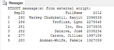

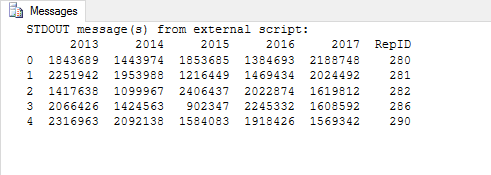

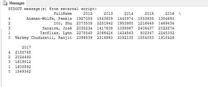
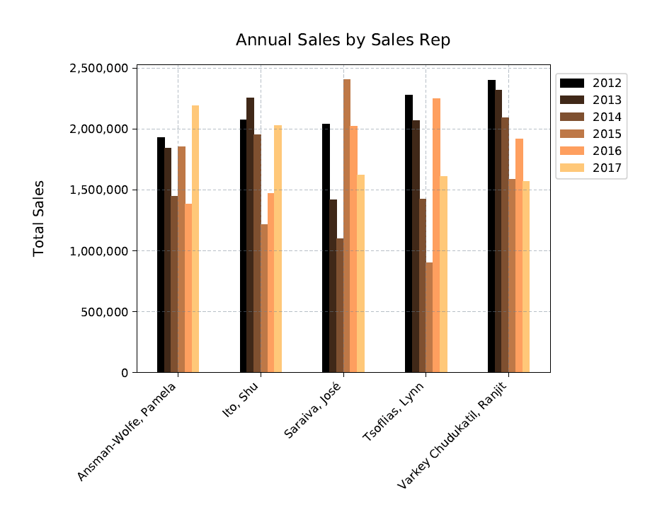
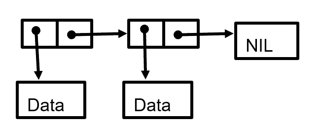
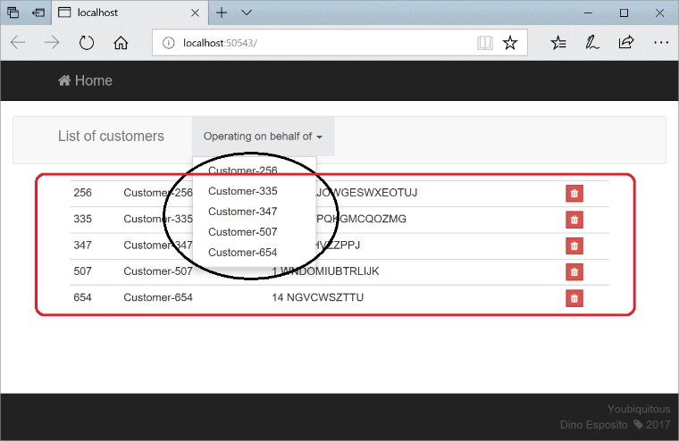
 Politiker von Union und SPD fordern nach dem Dieselurteil andere Lösungen als die blaue Plakette. Der Bundesverkehrsminister bezeichnete diese als "kalte Enteignung".
 Zwei Väter lernen sich in der Kita kennen und erfinden ein Abspielgerät für Kinderhörbücher. Jetzt ist die Toniebox so begehrt, dass sie seit Monaten ausverkauft ist.
 Flirt oder Übergriff? Affäre oder Machtmissbrauch? Sexualität am Arbeitsplatz ist besonders heikel. Vor allem für die Frau, sagt der Sexualtherapeut Ulrich Clement.
 Bosch hat sich trotz des Engagements in der Elektromobilität gegen eine eigene Akkuzellenproduktion entschieden. Auch die Forschung für bessere Akkuzellen will das Unternehmen zurückfahren oder verkaufen. (Bosch, Technologie)


 Die Richter des Bundesgerichtshofs haben das bundesweit erste Mordurteil gegen zwei Berliner Raser für unzulässig erklärt. Sie sehen den Tötungsvorsatz nicht erfüllt.


 Dieselfahrverbote in deutschen Städten sind künftig möglich, doch die Bundesregierung will sie weiter verhindern. Auch der Mittelstand warnt vor den Folgen von Verboten.