Nosimpler

Some people hear voices that others do not, but only some of those people seek treatment. Using a Pavlovian learning task, we induced conditioned hallucinations in four groups of people who differed orthogonally in their voice-hearing and treatment-seeking statuses. People who hear voices were significantly more susceptible to the effect. Using functional neuroimaging and computational modeling of perception, we identified processes that differentiated voice-hearers from non–voice-hearers and treatment-seekers from non–treatment-seekers and characterized a brain circuit that mediated the conditioned hallucinations. These data demonstrate the profound and sometimes pathological impact of top-down cognitive processes on perception and may represent an objective means to discern people with a need for treatment from those without.

The complete connectome of a learning and memory centre in an insect brain

Nature 548, 7666 (2017). doi:10.1038/nature23455

Authors: Katharina Eichler, Feng Li, Ashok Litwin-Kumar, Youngser Park, Ingrid Andrade, Casey M. Schneider-Mizell, Timo Saumweber, Annina Huser, Claire Eschbach, Bertram Gerber, Richard D. Fetter, James W. Truman, Carey E. Priebe, L. F. Abbott, Andreas S. Thum, Marta Zlatic & Albert Cardona

Associating stimuli with positive or negative reinforcement is essential for survival, but a complete wiring diagram of a higher-order circuit supporting associative memory has not been previously available. Here we reconstruct one such circuit at synaptic resolution, the Drosophila larval mushroom body. We find

Researchers have made a radio-frequency identification device that fits inside a cell.

[Physics] Published Wed Jul 26, 2017

Andrey Nikolaevich Kolmogorov was one of the giants of 20th-century mathematics.  I’ve always found it amazing that the same man was responsible both for establishing the foundations of classical probability theory in the 1930s, and also for co-inventing the theory of algorithmic randomness (a.k.a. Kolmogorov complexity) in the 1960s, which challenged the classical foundations, by holding that it is possible after all to talk about the entropy of an individual object, without reference to any ensemble from which the object was drawn.  Incredibly, going strong into his eighties, Kolmogorov then pioneered the study of “sophistication,” which amends Kolmogorov complexity to assign low values both to “simple” objects and “random” ones, and high values only to a third category of objects, which are “neither simple nor random.”  So, Kolmogorov was at the vanguard of the revolution, counter-revolution, and counter-counter-revolution.

But that doesn’t even scratch the surface of his accomplishments: he made fundamental contributions to topology and dynamical systems, and together with Vladimir Arnold, solved Hilbert’s thirteenth problem, showing that any multivariate continuous function can be written as a composition of continuous functions of two variables.  He mentored an awe-inspiring list of young mathematicians, whose names (besides Arnold) include Dobrushin, Dynkin, Gelfand, Martin-Löf, Sinai, and in theoretical computer science, our own Leonid Levin.  If that wasn’t enough, during World War II Kolmogorov applied his mathematical gifts to artillery problems, helping to protect Moscow from German bombardment.

Kolmogorov was private in his personal and political life, which might have had something to do with being gay, at a time and place when that was in no way widely accepted.  From what I’ve read—for example, in Gessen’s biography of Perelman—Kolmogorov seems to have been generally a model of integrity and decency.  He established schools for mathematically gifted children, which became jewels of the Soviet Union; one still reads about them with awe.  And at a time when Soviet mathematics was convulsed by antisemitism—with students of Jewish descent excluded from the top math programs for made-up reasons, sent instead to remote trade schools—Kolmogorov quietly protected Jewish researchers.

OK, but all this leaves a question.  Kolmogorov was a leading and admired Soviet scientist all through the era of Stalin’s purges, the Gulag, the KGB, the murders and disappearances and forced confessions, the show trials, the rewritings of history, the allies suddenly denounced as traitors, the tragicomedy of Lysenkoism.  Anyone as intelligent, individualistic, and morally sensitive as Kolmogorov would obviously have seen through the lies of his government, and been horrified by its brutality.  So then why did he utter nary a word in public against what was happening?

As far as I can tell, the answer is simply: because Kolmogorov knew better than to pick fights he couldn’t win.  He judged that he could best serve the cause of truth by building up an enclosed little bubble of truth, and protecting that bubble from interference by the Soviet system, and even making the bubble useful to the system wherever he could—rather than futilely struggling to reform the system, and simply making martyrs of himself and all his students for his trouble.

There’s a saying of Kolmogorov, which associates wisdom with keeping your mouth shut:

“Every mathematician believes that he is ahead of the others. The reason none state this belief in public is because they are intelligent people.”

There’s also a story that Kolmogorov loved to tell about himself, which presents math as a sort of refuge from the arbitrariness of the world: he said that he once studied to become a historian, but was put off by the fact that historians demanded ten different proofs for the same proposition, whereas in math, a single proof suffices.

There was also a dark side to political quietism.  In 1936, Kolmogorov joined other mathematicians in testifying against his former mentor in the so-called Luzin affair.  By many accounts, he did this because the police blackmailed him, by threatening to reveal his homosexual relationship with Pavel Aleksandrov.  On the other hand, while he was never foolish enough to take on Lysenko directly, Kolmogorov did publish a paper in 1940 courageously supporting Mendelian genetics.

---

It seems likely that in every culture, there have been truths, which moreover everyone knows to be true on some level, but which are so corrosive to the culture’s moral self-conception that one can’t assert them, or even entertain them seriously, without (in the best case) being ostracized for the rest of one’s life.  In the USSR, those truths were the ones that undermined the entire communist project: for example, that humans are not blank slates; that Mendelian genetics is right; that Soviet collectivized agriculture was a humanitarian disaster.  In our own culture, those truths are—well, you didn’t expect me to say, did you?

I’ve long been fascinated by the psychology of unspeakable truths.  Like, for any halfway perceptive person in the USSR, there must have been an incredible temptation to make a name for yourself as a daring truth-teller: so much low-hanging fruit!  So much to say that’s correct and important, and that best of all, hardly anyone else is saying!

But then one would think better of it.  It’s not as if, when you speak a forbidden truth, your colleagues and superiors will thank you for correcting their misconceptions.  Indeed, it’s not as if they didn’t already know, on some level, whatever you imagined yourself telling them.  In fact it’s often because they fear you might be right that the authorities see no choice but to make an example of you, lest the heresy spread more widely.  One corollary is that the more reasonably and cogently you make your case, the more you force the authorities’ hand.

But what’s the inner psychology of the authorities?  For some, it probably really is as cynical as the preceding paragraph makes it sound.  But for most, I doubt that.  I think that most authorities simply internalize the ruling ideology so deeply that they equate dissent with sin.  So in particular, the better you can ground your case in empirical facts, the craftier and more conniving a deceiver you become in their eyes, and hence the more virtuous they are for punishing you.  Someone who’s arrived at that point is completely insulated from argument: absent some crisis that makes them reevaluate their entire life, there’s no sense in even trying.  The question of whether or not your arguments have merit won’t even get entered upon, nor will the authority ever be able to repeat back your arguments in a form you’d recognize—for even repeating the arguments correctly could invite accusations of secretly agreeing with them.  Instead, the sole subject of interest will be you: who you think you are, what your motivations were to utter something so divisive and hateful.  And you have as good a chance of convincing authorities of your benign motivations as you’d have of convincing the Inquisition that, sure, you’re a heretic, but the good kind of heretic, the kind who rejects the divinity of Jesus but believes in niceness and tolerance and helping people.  To an Inquisitor, “good heretic” doesn’t parse any better than “round square,” and the very utterance of such a phrase is an invitation to mockery.  If the Inquisition had had Twitter, its favorite sentence would be “I can’t even.”

If it means anything to be a lover of truth, it means that anytime society finds itself stuck in one of these naked-emperor equilibriums—i.e., an equilibrium with certain facts known to nearly everyone, but severe punishments for anyone who tries to make those facts common knowledge—you hope that eventually society climbs its way out.  But crucially, you can hope this while also realizing that, if you tried singlehandedly to change the equilibrium, it wouldn’t achieve anything good for the cause of truth.  If iconoclasts simply throw themselves against a ruling ideology one by one, they can be picked off as easily as tribesmen charging a tank with spears, and each kill will only embolden the tank-gunners still further.  The charging tribesmen don’t even have the assurance that, if truth ultimately does prevail, then they’ll be honored as martyrs: they might instead end up like Ted Nelson babbling about hypertext in 1960, or H.C. Pocklington yammering about polynomial-time algorithms in 1917, nearly forgotten by history for being too far ahead of their time.

Does this mean that, like Winston Smith, the iconoclast simply must accept that 2+2=5, and that a boot will stamp on a human face forever?  No, not at all.  Instead the iconoclast can choose what I think of as the Kolmogorov option.  This is where you build up fortresses of truth in places the ideological authorities don’t particularly understand or care about, like pure math, or butterfly taxonomy, or irregular verbs.  You avoid a direct assault on any beliefs your culture considers necessary for it to operate.  You even seek out common ground with the local enforcers of orthodoxy.  Best of all is a shared enemy, and a way your knowledge and skills might be useful against that enemy.  For Kolmogorov, the shared enemy was the Nazis; for someone today, an excellent choice might be Trump, who’s rightly despised by many intellectual factions that spend most of their time despising each other.  Meanwhile, you wait for a moment when, because of social tectonic shifts beyond your control, the ruling ideology has become fragile enough that truth-tellers acting in concert really can bring it down.  You accept that this moment of reckoning might never arrive, or not in your lifetime.  But even if so, you could still be honored by future generations for building your local pocket of truth, and for not giving falsehood any more aid or comfort than was necessary for your survival.

---

When it comes to the amount of flak one takes for defending controversial views in public under one’s own name, I defer to almost no one.  For anyone tempted, based on this post, to call me a conformist or coward: how many times have you been denounced online, and from how many different corners of the ideological spectrum?  How many people have demanded your firing?   How many death threats have you received?  How many threatened lawsuits?  How many comments that simply say “kill yourself kike” or similar?  Answer and we can talk about cowardice.

But, yes, there are places even I won’t go, hills I won’t die on.  Broadly speaking:

• My Law is that, as a scientist, I’ll hold discovering and disseminating the truth to be a central duty of my life, one that overrides almost every other value.  I’ll constantly urge myself to share what I see as the truth, even if it’s wildly unpopular, or makes me look weird, or is otherwise damaging to me.
• The Amendment to the Law is that I’ll go to great lengths not to hurt anyone else’s feelings: for example, by propagating negative stereotypes, or by saying anything that might discourage any enthusiastic person from entering science.  And if I don’t understand what is or isn’t hurtful, then I’ll defer to the leading intellectuals in my culture to tell me.  This Amendment often overrides the Law, causing me to bite my tongue.
• The Amendment to the Amendment is that, when pushed, I’ll stand by what I care about—such as free scientific inquiry, liberal Enlightenment norms, humor, clarity, and the survival of the planet and of family and friends and colleagues and nerdy misfits wherever they might be found.  So if someone puts me in a situation where there’s no way to protect what I care about without speaking a truth that hurts someone’s feelings, then I might speak the truth, feelings be damned.  (Even then, though, I’ll try to minimize collateral damage.)

---

When I see social media ablaze with this or that popular falsehood, I sometimes feel the “Galileo urge” washing over me.  I think: I’m a tenured professor with a semi-popular blog.  How can I look myself in the mirror, if I won’t use my platform and relative job safety to declare to the world, “and yet it moves”?

But then I remember that even Galileo weighed his options and tried hard to be prudent.  In his mind, the Dialogue Concerning the Two Chief World Systems actually represented a compromise (!).  Galileo never declared outright that the earth orbits the sun.  Instead, he put the Copernican doctrine, as a “possible view,” into the mouth of his character Salviati—only to have Simplicio “refute” Salviati, by the final dialogue, with the argument that faith always trumps reason, and that human beings are pathetically unequipped to deduce the plan of God from mere surface appearances.  Then, when that fig-leaf turned out not to be wide enough to fool the Church, Galileo quickly capitulated.  He repented of his error, and agreed never to defend the Copernican heresy again.  And he didn’t, at least not publicly.

Some have called Galileo a coward for that.  But the great David Hilbert held a different view.  Hilbert said that science, unlike religion, has no need for martyrs, because it’s based on facts that can’t be denied indefinitely.  Given that, Hilbert considered Galileo’s response to be precisely correct: in effect Galileo told the Inquisitors, hey, you’re the ones with the torture rack.  Just tell me which way you want it.  I can have the earth orbiting Mars and Venus in figure-eights by tomorrow if you decree it so.

Three hundred years later, Andrey Kolmogorov would say to the Soviet authorities, in so many words: hey, you’re the ones with the Gulag and secret police.  Consider me at your service.  I’ll even help you stop Hitler’s ideology from taking over the world—you’re 100% right about that one, I’ll give you that.  Now as for your own wondrous ideology: just tell me the dogma of the week, and I’ll try to make sure Soviet mathematics presents no threat to it.

There’s a quiet dignity to Kolmogorov’s (and Galileo’s) approach: a dignity that I suspect will be alien to many, but recognizable to those in the business of science.

---

Comment Policy: I welcome discussion about the responses of Galileo, Kolmogorov, and other historical figures to official ideologies that they didn’t believe in; and about the meta-question of how a truth-valuing person ought to behave when living under such ideologies.  In the hopes of maintaining a civil discussion, any comments that mention current hot-button ideological disputes will be ruthlessly deleted.

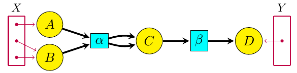
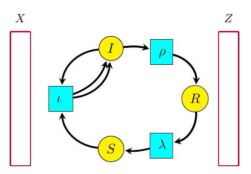
For a long time Blake Pollard and I have been working on ‘open’ chemical reaction networks: that is, networks of chemical reactions where some chemicals can flow in from an outside source, or flow out. The picture to keep in mind is something like this:

where the yellow circles are different kinds of chemicals and the aqua boxes are different reactions. The purple dots in the sets X and Y are ‘inputs’ and ‘outputs’, where certain kinds of chemicals can flow in or out.

Here’s our paper on this stuff:

• John Baez and Blake Pollard, A compositional framework for reaction networks, Reviews in Mathematical Physics 29, 1750028.

Blake and I gave talks about this stuff in Luxembourg this June, at a nice conference called Dynamics, thermodynamics and information processing in chemical networks. So, if you’re the sort who prefers talk slides to big scary papers, you can look at those:

• John Baez, The mathematics of open reaction networks.

• Blake Pollard, Black-boxing open reaction networks.

But I want to say here what we do in our paper, because it’s pretty cool, and it took a few years to figure it out. To get things to work, we needed my student Brendan Fong to invent the right category-theoretic formalism: ‘decorated cospans’. But we also had to figure out the right way to think about open dynamical systems!

In the end, we figured out how to first ‘gray-box’ an open reaction network, converting it into an open dynamical system, and then ‘black-box’ it, obtaining the relation between input and output flows and concentrations that holds in steady state. The first step extracts the dynamical behavior of an open reaction network; the second extracts its static behavior. And both these steps are functors!

Lawvere had the idea that the process of assigning ‘meaning’ to expressions could be seen as a functor. This idea has caught on in theoretical computer science: it’s called ‘functorial semantics’. So, what we’re doing here is applying functorial semantics to chemistry.

Now Blake has passed his thesis defense based on this work, and he just needs to polish up his thesis a little before submitting it. This summer he’s doing an internship at the Princeton branch of the engineering firm Siemens. He’s working with Arquimedes Canedo on ‘knowledge representation’.

But I’m still eager to dig deeper into open reaction networks. They’re a small but nontrivial step toward my dream of a mathematics of living systems. My working hypothesis is that living systems seem ‘messy’ to physicists because they operate at a higher level of abstraction. That’s what I’m trying to explore.

Here’s the idea of our paper.

The idea

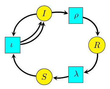
Reaction networks are a very general framework for describing processes where entities interact and transform int other entities. While they first showed up in chemistry, and are often called ‘chemical reaction networks’, they have lots of other applications. For example, a basic model of infectious disease, the ‘SIRS model’, is described by this reaction network:

We see here three types of entity, called species:

• : susceptible,
• : infected,
• : resistant.

We also have three `reactions’:

• : infection, in which a susceptible individual meets an infected one and becomes infected;
• : recovery, in which an infected individual gains resistance to the disease;
• : loss of resistance, in which a resistant individual becomes susceptible.

In general, a reaction network involves a finite set of species, but reactions go between complexes, which are finite linear combinations of these species with natural number coefficients. The reaction network is a directed graph whose vertices are certain complexes and whose edges are called reactions.

If we attach a positive real number called a rate constant to each reaction, a reaction network determines a system of differential equations saying how the concentrations of the species change over time. This system of equations is usually called the rate equation. In the example I just gave, the rate equation is

Here and are the rate constants for the three reactions, and now stand for the concentrations of the three species, which are treated in a continuum approximation as smooth functions of time:

The rate equation can be derived from the law of mass action, which says that any reaction occurs at a rate equal to its rate constant times the product of the concentrations of the species entering it as inputs.

But a reaction network is more than just a stepping-stone to its rate equation! Interesting qualitative properties of the rate equation, like the existence and uniqueness of steady state solutions, can often be determined just by looking at the reaction network, regardless of the rate constants. Results in this direction began with Feinberg and Horn’s work in the 1960’s, leading to the Deficiency Zero and Deficiency One Theorems, and more recently to Craciun’s proof of the Global Attractor Conjecture.

In our paper, Blake and I present a ‘compositional framework’ for reaction networks. In other words, we describe rules for building up reaction networks from smaller pieces, in such a way that its rate equation can be figured out knowing those those of the pieces. But this framework requires that we view reaction networks in a somewhat different way, as ‘Petri nets’.

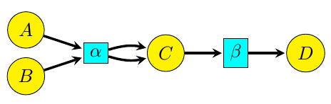
Petri nets were invented by Carl Petri in 1939, when he was just a teenager, for the purposes of chemistry. Much later, they became popular in theoretical computer science, biology and other fields. A Petri net is a bipartite directed graph: vertices of one kind represent species, vertices of the other kind represent reactions. The edges into a reaction specify which species are inputs to that reaction, while the edges out specify its outputs.

You can easily turn a reaction network into a Petri net and vice versa. For example, the reaction network above translates into this Petri net:

Beware: there are a lot of different names for the same thing, since the terminology comes from several communities. In the Petri net literature, species are called places and reactions are called transitions. In fact, Petri nets are sometimes called ‘place-transition nets’ or ‘P/T nets’. On the other hand, chemists call them ‘species-reaction graphs’ or ‘SR-graphs’. And when each reaction of a Petri net has a rate constant attached to it, it is often called a ‘stochastic Petri net’.

While some qualitative properties of a rate equation can be read off from a reaction network, others are more easily read from the corresponding Petri net. For example, properties of a Petri net can be used to determine whether its rate equation can have multiple steady states.

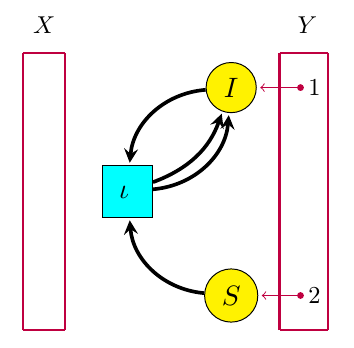
Petri nets are also better suited to a compositional framework. The key new concept is an ‘open’ Petri net. Here’s an example:

The box at left is a set X of ‘inputs’ (which happens to be empty), while the box at right is a set Y of ‘outputs’. Both inputs and outputs are points at which entities of various species can flow in or out of the Petri net. We say the open Petri net goes from X to Y. In our paper, we show how to treat it as a morphism in a category we call .

Given an open Petri net with rate constants assigned to each reaction, our paper explains how to get its ‘open rate equation’. It’s just the usual rate equation with extra terms describing inflows and outflows. The above example has this open rate equation:

Here are arbitrary smooth functions describing outflows as a function of time.

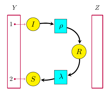
Given another open Petri net for example this:

it will have its own open rate equation, in this case

Here are arbitrary smooth functions describing inflows as a function of time. Now for a tiny bit of category theory: we can compose and by gluing the outputs of to the inputs of This gives a new open Petri net as follows:

But this open Petri net has an empty set of inputs, and an empty set of outputs! So it amounts to an ordinary Petri net, and its open rate equation is a rate equation of the usual kind. Indeed, this is the Petri net we have already seen.

As it turns out, there’s a systematic procedure for combining the open rate equations for two open Petri nets to obtain that of their composite. In the example we’re looking at, we just identify the outflows of with the inflows of (setting and ) and then add the right hand sides of their open rate equations.

The first goal of our paper is to precisely describe this procedure, and to prove that it defines a functor

from to a category where the morphisms are ‘open dynamical systems’. By a dynamical system, we essentially mean a vector field on which can be used to define a system of first-order ordinary differential equations in variables. An example is the rate equation of a Petri net. An open dynamical system allows for the possibility of extra terms that are arbitrary functions of time, such as the inflows and outflows in an open rate equation.

In fact, we prove that and are symmetric monoidal categories and that is a symmetric monoidal functor. To do this, we use Brendan Fong’s theory of ‘decorated cospans’.

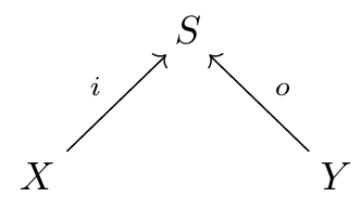
Decorated cospans are a powerful general tool for describing open systems. A cospan in any category is just a diagram like this:

We are mostly interested in cospans in the category of finite sets and functions between these. The set , the so-called apex of the cospan, is the set of states of an open system. The sets and are the inputs and outputs of this system. The legs of the cospan, meaning the morphisms and describe how these inputs and outputs are included in the system. In our application, is the set of species of a Petri net.

For example, we may take this reaction network:

treat it as a Petri net with :

and then turn that into an open Petri net by choosing any finite sets and maps , , for example like this:

(Notice that the maps including the inputs and outputs into the states of the system need not be one-to-one. This is technically useful, but it introduces some subtleties that I don’t feel like explaining right now.)

An open Petri net can thus be seen as a cospan of finite sets whose apex is ‘decorated’ with some extra information, namely a Petri net with as its set of species. Fong’s theory of decorated cospans lets us define a category with open Petri nets as morphisms, with composition given by gluing the outputs of one open Petri net to the inputs of another.

We call the functor

gray-boxing because it hides some but not all the internal details of an open Petri net. (In the paper we draw it as a gray box, but that’s too hard here!)

We can go further and black-box an open dynamical system. This amounts to recording only the relation between input and output variables that must hold in steady state. We prove that black-boxing gives a functor

(yeah, the box here should be black, and in our paper it is). Here is a category where the morphisms are semi-algebraic relations between real vector spaces, meaning relations defined by polynomials and inequalities. This relies on the fact that our dynamical systems involve algebraic vector fields, meaning those whose components are polynomials; more general dynamical systems would give more general relations.

That semi-algebraic relations are closed under composition is a nontrivial fact, a spinoff of the Tarski–Seidenberg theorem. This says that a subset of defined by polynomial equations and inequalities can be projected down onto , and the resulting set is still definable in terms of polynomial identities and inequalities. This wouldn’t be true if we didn’t allow inequalities. It’s neat to see this theorem, important in mathematical logic, showing up in chemistry!

Structure of the paper

Okay, now you’re ready to read our paper! Here’s how it goes:

In Section 2 we review and compare reaction networks and Petri nets. In Section 3 we construct a symmetric monoidal category where an object is a finite set and a morphism is an open reaction network (or more precisely, an isomorphism class of open reaction networks). In Section 4 we enhance this construction to define a symmetric monoidal category where the transitions of the open reaction networks are equipped with rate constants. In Section 5 we explain the open dynamical system associated to an open reaction network, and in Section 6 we construct a symmetric monoidal category of open dynamical systems. In Section 7 we construct the gray-boxing functor

In Section 8 we construct the black-boxing functor

We show both of these are symmetric monoidal functors.

Finally, in Section 9 we fit our results into a larger ‘network of network theories’. This is where various results in various papers I’ve been writing in the last few years start assembling to form a big picture! But this picture needs to grow….

In apparent contradiction to the laws of thermodynamics, Maxwell’s demon is able to cyclically extract work from a system in contact with a thermal bath, exploiting the information about its microstate. The resolution of this paradox required the insight that an intimate relationship exists between information and thermodynamics. Here, we...

Last week I organized a workshop on the future of academic publication. My point was that our current system, based on private pre-publication peer review, is archaic. I noted that the way the peer review system is currently organized (where external reviewers judge both the quality of the science and the interest for the journal) represents just a few decades in the history of science. It can hardly qualify as the way science is or should be done. It is a historical feature. For example, only one of Einstein’s papers was formally peer-reviewed; Crick & Watson’s DNA paper was not formally peer-reviewed. Many journals introduced external peer review in the 1960s or 1970s to deal with the growth in the number and variety of submissions (see e.g. Baldwin, 2015); before that, editors would decide whether to publish the papers they received, depending on the number of pages they could print.

Given the possibilities that offers the internet, it seems that there is no reason anymore to couple the two current roles of peer review: editorial selection and scientific discussion. One could simply share their work online, get feedback from the community to discuss the work, and then let people recommend papers to their colleagues and compile all sorts of reader’s digests. No time wasted in multiple submissions, no prestige misattributed to publications in glamour journals, who do not do a better a job than any other journal at pointing errors and frauds. Just the science and the public discussion of science.

But there is a lot of resistance to this idea, namely the idea that papers should be formally approved by peer reviewers before they are published. Because otherwise, so many people claim, the scientific world would be polluted by all sorts of unverified claims. It would not be science anymore, just gossip. I have attributed this attitude to conservatism, first because as noted above this system is a rather recent addition to the scientific enterprise, and second because papers are published before peer review. We call those “preprints”, but really these are scientific papers made public, so by definition they are published. I follow the preprints in my field and I don’t see any particular loss in quality.

However, I think I was missing a key element. The more profound reason why many people, in particular experimental biologists, are so attached to peer review is in my view that they hold naive philosophical views about the notion of truth in science. A paper should be peer-reviewed because otherwise you can’t cite it as a true fact. Peer review validates science, thanks to experts who make sure that the claims of the authors are actually true. Of course it can go wrong and reviewers might miss something, but it is the purpose of peer review. This view is reflected in the tendency, especially in biology journals, to choose titles that look like established truths: “Hunger is controlled by HGRase”, instead of “The molecular control of hunger”. Scientists and journalists can then write revealed truths with a verse reference, such as “Hunger is controlled by HGRase (McDonald et al., 2017)”.

The great misunderstanding is that truth is a notion that applies to logical propositions (for example, mathematical theorems), not to empirical claims. This has been well argued by Popper, for example. Truth is by nature a theoretical concept. Everything said is said with words, and in this sense it always refers to theoretical concepts. One can only judge whether observations are congruent with the meaning attributed to the words, and that meaning necessarily has a theoretical nature. There is no such thing as an “established fact”. This is so even of what we might consider as direct observations. Take for example the claim “The resting potential of neurons is -70 mV”. This is a theoretical statement. Why? First, because to establish it, I have recorded a number of neurons. If you test it, it will be on a different neuron, which I have not measured. So I am making a theoretical claim. Probably, I also tested my neurons with a particular method (not mentioning a particular region and species). But my claim makes no reference to the method by which I have made the inference. That would be the “methods” part of my paper, not the conclusion, and when you cite my paper, you will cite it because of the conclusion, the “established fact”, you will not be referring to the methods, which you consider are the means to establish the fact. It is the role of the reviewers to check the methods, to check that they do establish the fact.

But these are trivial remarks. It is not just that the method matters. The very notion of an observation always implicitly relies on a theoretical background. When I say that the resting potential is -70 mV, I mean that there is a potential difference of -70 mV across the membrane. But that’s not what I measure. I measure the difference in potential between some point outside the cell and the inside of a patch pipette whose solution is in contact with the cell’s inside. So I am assuming the potential is the same in all points of the cytosol, even though I have not tested it. I am also implicitly modeling the cytosol as a solution, even though the reality is more complex than that, given the mass of charged proteins in it. I am assuming that the extracellular potential is constant. I am assuming that my pipette solution reasonably matches the actual cytosol solution, given that “solution” is only a convenient model. I am implicitly making all sorts of theoretical assumptions, which have a lot of empirical support but are still of a theoretical nature.

I have tried with this example to show that even a very simple “fact” is actually a theoretical proposition, with many layers of assumptions. But of course in general, papers typically make claims that rely less firmly on accepted theoretical grounds, since they must be “novel”. So it is never the case that a paper definitely proves its conclusions. Because conclusions have a theoretical nature, all that can be checked is whether observations are consistent with the authors’ interpretation.

So the goal of peer review can’t be to establish the truth. If it were the case, then why would reviewers ever disagree? They disagree because they cannot actually judge whether a claim is true; they can only say whether they are personally convinced. This makes the current peer review system extremely poor, because all the information we get is: two anonymous people were convinced (and maybe others were not, but we’ll never find out). What would be more useful would be to have an open public discussion, with criticisms, qualifications and alternative interpretations fully disclosed for anyone to read and make their own opinion. In such a system, the notion of a stamp of approval on a paper would simply be absurd; why hide the disapprovals? There is the paper, and there is the scientific discussion of the paper, and that is all there needs to be.

There is some concern these days that peer reviewed research is unreliable. Well, science is unreliable. That is almost what defines it: it can be criticized and revised. Seeing peer review as the system that establishes the scientific truth is not only a historical error, it is a great philosophical error, and a dangerous bureaucratic view of science. We don’t need editorial decisions based on peer review. We need free publication (we have it) and we need open scientific discussion (it’s coming). That’s all we need.

I’ve just uploaded to the arXiv my paper “On the universality of the incompressible Euler equation on compact manifolds“, submitted to Discrete and Continuous Dynamical Systems. This is a variant of my recent paper on the universality of potential well dynamics, but instead of trying to embed dynamical systems into a potential well , here we try to embed dynamical systems into the incompressible Euler equations

on a Riemannian manifold . (One is particularly interested in the case of flat manifolds , particularly or , but for the main result of this paper it is essential that one is permitted to consider curved manifolds.) This system, first studied by Ebin and Marsden, is the natural generalisation of the usual incompressible Euler equations to curved space; it can be viewed as the formal geodesic flow equation on the infinite-dimensional manifold of volume-preserving diffeomorphisms on (see this previous post for a discussion of this in the flat space case).

The Euler equations can be viewed as a nonlinear equation in which the nonlinearity is a quadratic function of the velocity field . It is thus natural to compare the Euler equations with quadratic ODE of the form

where is the unknown solution, and is a bilinear map, which we may assume without loss of generality to be symmetric. One can ask whether such an ODE may be linearly embedded into the Euler equations on some Riemannian manifold , which means that there is an injective linear map from to smooth vector fields on , as well as a bilinear map to smooth scalar fields on , such that the map takes solutions to (2) to solutions to (1), or equivalently that

for all .

For simplicity let us restrict to be compact. There is an obvious necessary condition for this embeddability to occur, which comes from energy conservation law for the Euler equations; unpacking everything, this implies that the bilinear form in (2) has to obey a cancellation condition

for some positive definite inner product on . The main result of the paper is the converse to this statement: if is a symmetric bilinear form obeying a cancellation condition (3), then it is possible to embed the equations (2) into the Euler equations (1) on some Riemannian manifold ; the catch is that this manifold will depend on the form and on the dimension (in fact in the construction I have, is given explicitly as , with a funny metric on it that depends on ).

As a consequence, any finite dimensional portion of the usual “dyadic shell models” used as simplified toy models of the Euler equation, can actually be embedded into a genuine Euler equation, albeit on a high-dimensional and curved manifold. This includes portions of the self-similar “machine” I used in a previous paper to establish finite time blowup for an averaged version of the Navier-Stokes (or Euler) equations. Unfortunately, the result in this paper does not apply to infinite-dimensional ODE, so I cannot yet establish finite time blowup for the Euler equations on a (well-chosen) manifold. It does not seem so far beyond the realm of possibility, though, that this could be done in the relatively near future. In particular, the result here suggests that one could construct something resembling a universal Turing machine within an Euler flow on a manifold, which was one ingredient I would need to engineer such a finite time blowup.

The proof of the main theorem proceeds by an “elimination of variables” strategy that was used in some of my previous papers in this area, though in this particular case the Nash embedding theorem (or variants thereof) are not required. The first step is to lessen the dependence on the metric by partially reformulating the Euler equations (1) in terms of the covelocity (which is a -form) instead of the velocity . Using the freedom to modify the dimension of the underlying manifold , one can also decouple the metric from the volume form that is used to obtain the divergence-free condition. At this point the metric can be eliminated, with a certain positive definiteness condition between the velocity and covelocity taking its place. After a substantial amount of trial and error (motivated by some “two-and-a-half-dimensional” reductions of the three-dimensional Euler equations, and also by playing around with a number of variants of the classic “separation of variables” strategy), I eventually found an ansatz for the velocity and covelocity that automatically solved most of the components of the Euler equations (as well as most of the positive definiteness requirements), as long as one could find a number of scalar fields that obeyed a certain nonlinear system of transport equations, and also obeyed a positive definiteness condition. Here I was stuck for a bit because the system I ended up with was overdetermined – more equations than unknowns. After trying a number of special cases I eventually found a solution to the transport system on the sphere, except that the scalar functions sometimes degenerated and so the positive definiteness property I wanted was only obeyed with positive semi-definiteness. I tried for some time to perturb this example into a strictly positive definite solution before eventually working out that this was not possible. Finally I had the brainwave to lift the solution from the sphere to an even more symmetric space, and this quickly led to the final solution of the problem, using the special orthogonal group rather than the sphere as the underlying domain. The solution ended up being rather simple in form, but it is still somewhat miraculous to me that it exists at all; in retrospect, given the overdetermined nature of the problem, relying on a large amount of symmetry to cut down the number of equations was basically the only hope.

Filed under: math.AP, math.DS, math.MG, paper Tagged: Euler equations, universality

Why I obsess about this stuff...

Proponents of self-driving cars say they'll make the world safer, but autonomous vehicles need to predict what bicyclists are going to do. Now researchers say part of the answer is to have bikes feed information to cars.

Just follow this logically about what they think their toys will require....

Erica Klarreich is one of the few science journalists who explains interesting things I don’t already know clearly enough so I can understand them. I recommend her latest article:

• Erica Klarreich, In game theory, no clear path to equilibrium, Quanta, 18 July 2017.

Economists like the concept of ‘Nash equilibrium’, but it’s problematic in some ways. This matters for society at large.

In a Nash equilibrium for a multi-player game, no player can improve their payoff by unilaterally changing their strategy. This doesn’t mean everyone is happy: it’s possible to be trapped in a Nash equilibrium where everyone is miserable, because anyone changing their strategy unilaterally would be even more miserable. (Think ‘global warming’.)

The great thing about Nash equilibria is that their meaning is easy to fathom, and they exist. John Nash won a Nobel prize for a paper proving that they exist. His paper was less than one page long. But he proved the existence of Nash equilibria for arbitrary multi-player games using a nonconstructive method: a fixed point theorem that doesn’t actually tell you how to find the equilibrium!

Given this, it’s not surprising that Nash equilibria can be hard to find. Last September a paper came out making this precise, in a strong way:

• Yakov Babichenko and Aviad Rubinstein, Communication complexity of approximate Nash equilibria.

The authors show there’s no guaranteed method for players to find even an approximate Nash equilibrium unless they tell each other almost everything about their preferences. This makes finding the Nash equilibrium prohibitively difficult to find when there are lots of players… in general. There are particular games where it’s not difficult, and that makes these games important: for example, if you’re trying to run a government well. (A laughable notion these days, but still one can hope.)

Klarreich’s article in Quanta gives a nice readable account of this work and also a more practical alternative to the concept of Nash equilibrium. It’s called a ‘correlated equilibrium’, and it was invented by the mathematician Robert Aumann in 1974. You can see an attempt to define it here:

• Wikipedia, Correlated equilibrium.

The precise mathematical definition near the start of this article is a pretty good example of how you shouldn’t explain something: it contains a big fat equation containing symbols not mentioned previously, and so on. By thinking about it for a while, I was able to fight my way through it. Someday I should improve it—and someday I should explain the idea here! But for now, I’ll just quote this passage, which roughly explains the idea in words:

The idea is that each player chooses their action according to their observation of the value of the same public signal. A strategy assigns an action to every possible observation a player can make. If no player would want to deviate from the recommended strategy (assuming the others don’t deviate), the distribution is called a correlated equilibrium.

According to Erica Klarreich it’s a useful notion. She even makes it sound revolutionary:

This might at first sound like an arcane construct, but in fact we use correlated equilibria all the time—whenever, for example, we let a coin toss decide whether we’ll go out for Chinese or Italian, or allow a traffic light to dictate which of us will go through an intersection first.

In [some] examples, each player knows exactly what advice the “mediator” is giving to the other player, and the mediator’s advice essentially helps the players coordinate which Nash equilibrium they will play. But when the players don’t know exactly what advice the others are getting—only how the different kinds of advice are correlated with each other—Aumann showed that the set of correlated equilibria can contain more than just combinations of Nash equilibria: it can include forms of play that aren’t Nash equilibria at all, but that sometimes result in a more positive societal outcome than any of the Nash equilibria. For example, in some games in which cooperating would yield a higher total payoff for the players than acting selfishly, the mediator can sometimes beguile players into cooperating by withholding just what advice she’s giving the other players. This finding, Myerson said, was “a bolt from the blue.”

(Roger Myerson is an economics professor at the University of Chicago who won a Nobel prize for his work on game theory.)

And even though a mediator can give many different kinds of advice, the set of correlated equilibria of a game, which is represented by a collection of linear equations and inequalities, is more mathematically tractable than the set of Nash equilibria. “This other way of thinking about it, the mathematics is so much more beautiful,” Myerson said.

While Myerson has called Nash’s vision of game theory “one of the outstanding intellectual advances of the 20th century,” he sees correlated equilibrium as perhaps an even more natural concept than Nash equilibrium. He has opined on numerous occasions that “if there is intelligent life on other planets, in a majority of them they would have discovered correlated equilibrium before Nash equilibrium.”

When it comes to repeated rounds of play, many of the most natural ways that players could choose to adapt their strategies converge, in a particular sense, to correlated equilibria. Take, for example, “regret minimization” approaches, in which before each round, players increase the probability of using a given strategy if they regret not having played it more in the past. Regret minimization is a method “which does bear some resemblance to real life — paying attention to what’s worked well in the past, combined with occasionally experimenting a bit,” Roughgarden said.

(Tim Roughgarden is a theoretical computer scientist at Stanford University.)

For many regret-minimizing approaches, researchers have shown that play will rapidly converge to a correlated equilibrium in the following surprising sense: after maybe 100 rounds have been played, the game history will look essentially the same as if a mediator had been advising the players all along. It’s as if “the [correlating] device was somehow implicitly found, through the interaction,” said Constantinos Daskalakis, a theoretical computer scientist at the Massachusetts Institute of Technology.

As play continues, the players won’t necessarily stay at the same correlated equilibrium — after 1,000 rounds, for instance, they may have drifted to a new equilibrium, so that now their 1,000-game history looks as if it had been guided by a different mediator than before. The process is reminiscent of what happens in real life, Roughgarden said, as societal norms about which equilibrium should be played gradually evolve.

In the kinds of complex games for which Nash equilibrium is hard to reach, correlated equilibrium is “the natural leading contender” for a replacement solution concept, Nisan said.

As Klarreich hints, you can find correlated equilibria using a technique called linear programming. That was proved here, I think:

• Christos H. Papadimitriou and Tim Roughgarden, Computing correlated equilibria in multi-player games, J. ACM 55 (2008), 14:1-14:29.

Do you know something about correlated equilibria that I should know? If so, please tell me!

Immunology: Nervous crosstalk to make antibodies

Nature 547, 7663 (2017). doi:10.1038/nature23097

Authors: Hai Qi

Immune cells called T cells help immune-system B cells mature to produce antibodies. This entails signalling between cells using the molecule dopamine — a surprising immunological role for this neurotransmitter. See Article p.318

The strange topology that is reshaping physics

Nature 547, 7663 (2017). http://www.nature.com/doifinder/10.1038/547272a

Author: Davide Castelvecchi

Topological effects might be hiding inside perfectly ordinary materials, waiting to reveal bizarre new particles or bolster quantum computing.

Merriam-Webster's Word of the Day for July 15, 2017 is:

copacetic • \koh-puh-SET-ik\  • adjective

: very satisfactory

Examples:

"... if you're going to be traveling with us it just wouldn't look too copacetic for you to be carrying that ratty old bag." — Christopher Paul Curtis, Bud, Not Buddy, 1999

"In terms of living standards we're now back to where we started which while not making us entirely copacetic is at least better than not having recovered as yet." — Tim Worstall, Forbes, 8 Aug. 2016

Did you know?

Theories about the origin of copacetic abound, but the facts about the word’s history are scant: it appears to have arisen in African-American slang in the southern U.S., possibly as early as the 1880s, with earliest known evidence of it in print dating only to 1919. Beyond that, we have only speculation. One theory is that the term is descended from Hebrew kol be sedher (or kol b’seder or chol b’seder), meaning “everything is in order.” That theory is problematic for a number of reasons, among them that in order for a Hebrew expression to have been adopted into English at that time it would have passed through Yiddish, and there is no evidence of the phrase in Yiddish dictionaries. Other theories trace copacetic to Creole coupèstique (“able to be coped with”), Italian cappo sotto (literally “head under,” figuratively “okay”), or Chinook jargon copacete (“everything’s all right”), but no evidence to substantiate any of these has been found. Another theory credits the coining of the word to Bill "Bojangles" Robinson, who used the word frequently and believed himself to be the coiner. Anecdotal recollections of the word’s use, however, predate his lifetime.

I occasionally come across a new piece of notation so good that it makes life easier by giving a better way to look at something. Some examples:

• Iverson introduced the notation [X] to mean 1 if X is true and 0 otherwise; so for example Σ_1≤n<x [n prime] is the number of primes less than x, and the unmemorable and confusing Kronecker delta function δ_n becomes [n=0]. (A similar convention is used in the C programming language.)

• The function taking x to x sin(x) can be denoted by x ↦ x sin(x). This has the same meaning as the lambda calculus notation λx.x sin(x) but seems easier to understand and use, and is less confusing than the usual convention of just writing x sin(x), which is ambiguous: it could also stand for a number.

• I find calculations with Homs and ⊗ easier to follow if I write Hom(A,B) as A→B. Similarly writing B^A for the set of functions from A to B is really confusing, and I find it much easier to write this set as A→B.

• Conway's notation for orbifolds almost trivializes the classification of wallpaper groups.

Has anyone come across any more similar examples of good notation that should be better known? (Excluding standard well known examples such as commutative diagrams, Hindu-Arabic numerals, etc.)

"A red palm weevil appears to strike a pugilistic stance, with its unusual antennae raised on either side of its elongated head." Macro photography specialist Javier Rupérez photographed the weevil in in his hometown of Almáchar, Spain

One of the Pictures of the Day at The Telegraph.

A century-old tenet in physics and engineering asserts that any type of system, having bandwidth , can interact with a wave over only a constrained time period t inversely proportional to the bandwidth (t· ~ 2). This law severely limits the generic capabilities of all types of resonant and wave-guiding systems in photonics, cavity quantum electrodynamics and optomechanics, acoustics, continuum mechanics, and atomic and optical physics but is thought to be completely fundamental, arising from basic Fourier reciprocity. We propose that this "fundamental" limit can be overcome in systems where Lorentz reciprocity is broken. As a system becomes more asymmetric in its transport properties, the degree to which the limit can be surpassed becomes greater. By way of example, we theoretically demonstrate how, in an astutely designed magnetized semiconductor heterostructure, the above limit can be exceeded by orders of magnitude by using realistic material parameters. Our findings revise prevailing paradigms for linear, time-invariant resonant systems, challenging the doctrine that high-quality resonances must invariably be narrowband and providing the possibility of developing devices with unprecedentedly high time-bandwidth performance.

Robust wireless power transfer using a nonlinear parity–time-symmetric circuit

Nature 546, 7658 (2017). doi:10.1038/nature22404

Authors: Sid Assawaworrarit, Xiaofang Yu & Shanhui Fan

Considerable progress in wireless power transfer has been made in the realm of non-radiative transfer, which employs magnetic-field coupling in the near field. A combination of circuit resonance and impedance transformation is often used to help to achieve efficient transfer of power over a predetermined distance of about the size of the resonators. The development of non-radiative wireless power transfer has paved the way towards real-world applications such as wireless powering of implantable medical devices and wireless charging of stationary electric vehicles. However, it remains a fundamental challenge to create a wireless power transfer system in which the transfer efficiency is robust against the variation of operating conditions. Here we propose theoretically and demonstrate experimentally that a parity–time-symmetric circuit incorporating a nonlinear gain saturation element provides robust wireless power transfer. Our results show that the transfer efficiency remains near unity over a distance variation of approximately one metre, without the need for any tuning. This is in contrast with conventional methods where high transfer efficiency can only be maintained by constantly tuning the frequency or the internal coupling parameters as the transfer distance or the relative orientation of the source and receiver units is varied. The use of a nonlinear parity–time-symmetric circuit should enable robust wireless power transfer to moving devices or vehicles.

Implantation of electrical probes into the brain has been central to both neuroscience research and biomedical applications, although conventional probes induce gliosis in surrounding tissue. We recently reported ultraflexible open mesh electronics implanted into rodent brains by syringe injection that exhibit promising chronic tissue response and recording stability. Here we...

Author(s): Adhip Agarwala and Vijay B. Shenoy

Topological insulators, so far only identified in materials with an ordered crystal structure, could potentially be found in amorphous materials.

[Phys. Rev. Lett. 118, 236402] Published Thu Jun 08, 2017

Collective motion in biology is often modelled as a dynamical system, in which individuals are represented as particles whose interactions are determined by the current state of the system. Many animals, however, including humans, have predictive capabilities, and presumably base their behavioural decisions---at least partially---upon an anticipated state of their environment. We explore a minimal version of this idea in the context of particles that interact according to a pairwise potential. Anticipation enters the picture by calculating the interparticle forces from linear extrapolations of the particle positions some time $\tau$ into the future. Simulations show that for intermediate values of $\tau$, compared to a transient time scale defined by the potential and the initial conditions, the particles form rotating clusters in which the particles are arranged in a hexagonal pattern. Analysis of the system shows that anticipation induces energy dissipation and we show that the kinetic energy asymptotically decays as $1/t$. Furthermore, we show that the angular momentum is not necessarily conserved for $\tau >0$, and that asymmetries in the initial condition therefore can cause rotational movement. These results suggest that anticipation could play an important role in collective behaviour, since it induces pattern formation and stabilises the dynamics of the system.

Ring attractors are a class of recurrent networks hypothesized to underlie the representation of heading direction. Such network structures, schematized as a ring of neurons whose connectivity depends on their heading preferences, can sustain a bump-like activity pattern whose location can be updated by continuous shifts along either turn direction. We recently reported that a population of fly neurons represents the animal’s heading via bump-like activity dynamics. We combined two-photon calcium imaging in head-fixed flying flies with optogenetics to overwrite the existing population representation with an artificial one, which was then maintained by the circuit with naturalistic dynamics. A network with local excitation and global inhibition enforces this unique and persistent heading representation. Ring attractor networks have long been invoked in theoretical work; our study provides physiological evidence of their existence and functional architecture.

Nature Neuroscience 20, 886 (2017). doi:10.1038/nn.4548

Authors: Zhisong He, Dingding Han, Olga Efimova, Patricia Guijarro, Qianhui Yu, Anna Oleksiak, Shasha Jiang, Konstantin Anokhin, Boris Velichkovsky, Stefan Grünewald & Philipp Khaitovich

Expressive eye widening (as in fear) and eye narrowing (as in disgust) are associated with opposing optical consequences and serve opposing perceptual functions. Lee and Anderson suggest that the opposing effects of eye widening and narrowing on the expresser’s visual perception have been socially co-opted to denote opposing mental states of sensitivity and discrimination, respectively, such that opposing complex mental states may originate from this simple perceptual opposition. Their abstract:

Human eyes convey a remarkable variety of complex social and emotional information. However, it is unknown which physical eye features convey mental states and how that came about. In the current experiments, we tested the hypothesis that the receiver’s perception of mental states is grounded in expressive eye appearance that serves an optical function for the sender. Specifically, opposing features of eye widening versus eye narrowing that regulate sensitivity versus discrimination not only conveyed their associated basic emotions (e.g., fear vs. disgust, respectively) but also conveyed opposing clusters of complex mental states that communicate sensitivity versus discrimination (e.g., awe vs. suspicion). This sensitivity-discrimination dimension accounted for the majority of variance in perceived mental states (61.7%). Further, these eye features remained diagnostic of these complex mental states even in the context of competing information from the lower face. These results demonstrate that how humans read complex mental states may be derived from a basic optical principle of how people see.

Here’s a video of the talk I gave at the Stanford Complexity Group:

You can see slides here:

• Biology as information dynamics.

Abstract. If biology is the study of self-replicating entities, and we want to understand the role of information, it makes sense to see how information theory is connected to the ‘replicator equation’ — a simple model of population dynamics for self-replicating entities. The relevant concept of information turns out to be the information of one probability distribution relative to another, also known as the Kullback–Liebler divergence. Using this we can get a new outlook on free energy, see evolution as a learning process, and give a clearer, more general formulation of Fisher’s fundamental theorem of natural selection.

I’d given a version of this talk earlier this year at a workshop on Quantifying biological complexity, but I’m glad this second try got videotaped and not the first, because I was a lot happier about my talk this time. And as you’ll see at the end, there were a lot of interesting questions.

Excerpts from an interesting article in this month's The Atlantic:

Our ability to know the price of anything, anytime, anywhere, has given us, the consumers, so much power that retailers—in a desperate effort to regain the upper hand, or at least avoid extinction—are now staring back through the screen. They are comparison shopping us...

The price of a can of soda in a vending machine can now vary with the temperature outside. The price of the headphones Google recommends may depend on how budget-conscious your web history shows you to be, one study found. For shoppers, that means price—not the one offered to you right now, but the one offered to you 20 minutes from now, or the one offered to me, or to your neighbor—may become an increasingly unknowable thing...

Four researchers in Catalonia tried to answer the question with dummy computers that mimicked the web-browsing patterns of either “affluent” or “budget conscious” customers for a week. When the personae went “shopping,” they weren’t shown different prices for the same goods. They were shown different goods. The average price of the headphones suggested for the affluent personae was four times the price of those suggested for the budget-conscious personae. Another experiment demonstrated a more direct form of price discrimination: Computers with addresses in greater Boston were shown lower prices than those in more-remote parts of Massachusetts on identical goods...

More at the link.

[cat picture]

Kevin Lewis pointed me to this article:

There are several methods for building hype. The wealth of currently available public relations techniques usually forces the promoter to judge, a priori, what will likely be the best method. Meta-hype is a methodology that facilitates this decision by combining all identified hype algorithms pertinent for a particular promotion problem. Meta-hype generates a final press release that is at least as good as any of the other models considered for hyping the claim. The overarching aim of this work is to introduce meta-hype to analysts and practitioners. This work compares the performance of journal publication, preprints, blogs, twitter, Ted talks, NPR, and meta-hype to predict successful promotion. A nationwide database including 89,013 articles, tweets, and news stories. All algorithms were evaluated using the total publicity value (TPV) in a test sample that was not included in the training sample used to fit the prediction models. TPV for the models ranged between 0.693 and 0.720. Meta-hype was superior to all but one of the algorithms compared. An explanation of meta-hype steps is provided. Meta-hype is the first step in targeted hype, an analytic framework that yields double hyped promotion with fewer assumptions than the usual publicity methods. Different aspects of meta-hype depending on the context, its function within the targeted promotion framework, and the benefits of this methodology in the addiction to extreme claims are discussed.

I can’t seem to find the link right now, but you get the idea.

P.S. The above is a parody of the abstract of a recent article on “super learning” by Acion et al. I did not include a link because the parody was not supposed to be a criticism of the content of the paper in any way; I just thought some of the wording in the abstract was kinda funny. Indeed, I thought I’d disguised the abstract enough that no one would make the connection but I guess Google is more powerful than I’d realized.

But this discussion by Erin in the comment thread revealed that some people were taking this post in a way I had not intended. So I added this comment.

tl;dr: I’m not criticizing the content of the Acion et al. paper in any way, and the above post was not intended to be seen as such a criticism.

The post The meta-hype algorithm appeared first on Statistical Modeling, Causal Inference, and Social Science.

Journal of Cognitive Neuroscience, Volume 29, Issue 10, Page 1684-1698, October 2017.

The post Las Vegas average is over no arbitrage condition appeared first on Marginal REVOLUTION.