Ricardo Ceneviva

Last week, I posted about statisticians’ constant battle against the belief that the p-value associated (for example) with a regression coefficient is equal to the probability that the null hypothesis is true, for a null hypothesis that beta is zero or negative. I argued that (despite our long pedagogical practice) there are, in fact, many situations where this interpretation of the p-value is actually the correct one (or at least close: it’s our rational belief about this probability, given the observed evidence).

In brief, according to Bayes’ rule,   equals , or . Under the prior belief that all values of are equally likely a priori, this expression reduces to ; this is just the p-value (where we consider starting with the likelihood density conditional on  with a horizontal line at , and then sliding the entire distribution to the left adding up the area swept under the likelihood by that line).

As I also explained in the earlier post, everything about my training and teaching experience tells me that this way lies madness. But despite the apparent unorthodoxy of the statement–that the p-value really is the probability that the null hypothesis is true, at least under some circumstances–this is a well-known and non-controversial result (see Greenland and Poole’s 2013 article in Epidemiology). Even better, it is easily verified with a simple R simulation.

rm(list=ls())
set.seed(12391)
require(hdrcde)
require(Bolstad)

b<-runif(15000, min=-2, max=2)
hist(b)

t<-c()
for(i in 1:length(b)){

 x<-runif(500)
 y<-x*b[i]+rnorm(500, sd=2)

 t[i]<-summary(lm(y~x))$coefficients[2,3]

}

b.eval<-seq(from=-1, to=2, by=0.005)
t.cde <- cde(t, b, x.name="t statistic", y.name="beta coefficient", y.margin=b.eval, x.margin=qt(0.95, df=498))
plot(t.cde)
abline(v=0, lty=2)

den.val<-cde(t, b, y.margin=b.eval, x.margin=qt(0.95, df=498))$z
sintegral(x=b.eval[which(b.eval<=0)], fx=den.val[which(b.eval<=0)])$value

This draws 15,000 “true” beta values from the uniform density from -2 to 2, generates a 500 observation data set for each one out of , estimates a correctly specified regression on the data set, and records the estimated t-statistic on the estimate of beta. The plotted figure below shows the estimated conditional density of true beta values given ; using Simpson’s rule integration, I calculated that the probability that given is 5.68%. This is very close to the theoretical 5% expectation for a one-tailed test of the null that .

The trouble, at least from where I stand, is that I wouldn’t want to substitute one falsehood (that the p-value is never equal to the probability that the null hypothesis is true) for another (that the p-value is always a great estimate of the probability that the null hypothesis is true). What am I supposed to tell my students?

Well, I have an idea. We’re very used to teaching the idea that, for example, OLS Regression is the best linear unbiased estimator for regression coefficients–but only when certain assumptions are true. We could teach students that p-values are a good estimate of the probability that the null hypothesis is true, but only when certain assumptions are true. Those assumptions include:

• The null hypothesis is an interval, not a point null. One-tailed alternative hypotheses (implying one-tailed nulls) are the most obvious candidates for this interpretation.
• The population of coefficients out of which this particular relationship’s is drawn (a.k.a. the prior belief distribution) must be uniformly distributed over the real number line (a.k.a. an uninformative improper prior). This means that we must presume total ignorance of the phenomenon before this study, and the justifiable belief in ignorance that is just as probable as a priori.
• Whatever other assumptions are needed to sustain the validity of parameters estimated by the model. This just says that if we’re going to talk about the probability that the null hypothesis about a parameter is true, we have to have a belief that this parameter is a valid estimator of some aspect of the DGP.  We might classify the Classical Linear Normal Regression Model assumptions underlying OLS linear models under this rubric.

When one or more of these assumptions is not true, p-value estimates could well be a biased estimate of the probability that the null hypothesis is true. What will this bias look like, and how bad will it be? We can demonstrate with some R simulations. As before, we assume a correctly specified linear model between two variables, , with an interval null hypothesis that .

The first set of simulations keeps the uniform distribution of that I used from the first simulation, but adds in a spike at of varying height. This is equivalent to saying that there is some fixed probability that , and one minus that probability that lies anywhere between -2 and 2. I vary the height of the spike between 0 and 0.8.

rm(list=ls())
set.seed(12391)

require(hdrcde)
require(Bolstad)

spike.prob<-c(0, 0.1, 0.2, 0.3, 0.4, 0.5, 0.6, 0.7, 0.8)
calc.prob<-c()
for(j in 1:length(spike.prob)){

cat("Currently Calculating for spike probability = ", spike.prob[j], "\n")
b.temp<-runif(15000, min=-2, max=2)
b<-ifelse(runif(15000)<spike.prob[j], 0, b.temp)

t<-c()
for(i in 1:length(b)){

x<-runif(500)
y<-x*b[i]+rnorm(500, sd=2)

t[i]<-summary(lm(y~x))$coefficients[2,3]

}

b.eval<-seq(from=-2, to=2, by=0.005)
den.val<-cde(t, b, y.margin=b.eval, x.margin=qt(0.95, df=498))$z
calc.prob[j]<-sintegral(x=b.eval[which(b.eval<=0)], fx=den.val[which(b.eval<=0)])$value

}

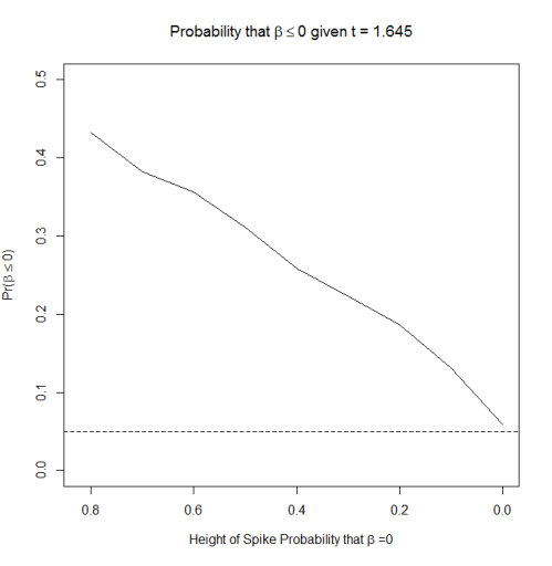
plot(calc.prob~spike.prob, type="l", xlim=c(0.82,0), ylim=c(0, 0.5), main=expression(paste("Probability that ", beta <=0, " given ", t>=1.645)), xlab=expression(paste("Height of Spike Probability that ", beta, " =0")), ylab=expression(paste("Pr(", beta <= 0,")")))
abline(h=0.05, lty=2)

The results are depicted in the plot below; the x-axis is reversed to put higher spikes on the left hand side and lower spikes on the right hand side. As you can see, the greater the chance that (that there is no relationship between x and y in a regression), the higher the probability that given that is statistically significant (the dotted line is at , the theoretical expectation). The distance between the solid and dotted line is the “bias” in the estimate of the probability that the null hypothesis is true; the p-value is almost always extremely overconfident. That is, seeing a p-value of 0.05 and concluding that there was a 5% chance that the null was true would substantially underestimate the true probability that there was no relationship between x and y.

The second set of simulations replaces the uniform distribution of true values with a normal distribution, where we center each distribution on zero but vary its standard deviation from wide to narrow.

rm(list=ls())
set.seed(12391)

require(hdrcde)
require(Bolstad)

sd.vec<-c(2, 1, 0.5, 0.25, 0.1)
calc.prob<-c()
for(j in 1:length(sd.vec)){

  cat("Currently Calculating for sigma = ", sd.vec[j], "\n")
  b<-rnorm(15000, mean=0, sd=sd.vec[j])

  t<-c()
  for(i in 1:length(b)){

    x<-runif(500)
    y<-x*b[i]+rnorm(500, sd=2)

    t[i]<-summary(lm(y~x))$coefficients[2,3]

  }

  b.eval<-seq(from=-3*sd.vec[j], to=3*sd.vec[j], by=0.005)
  den.val<-cde(t, b, y.margin=b.eval, x.margin=qt(0.95, df=498))$z
  calc.prob[j]<-sintegral(x=b.eval[which(b.eval<=0)], fx=den.val[which(b.eval<=0)])$value

}

plot(calc.prob~sd.vec, type="l", xlim=c(0, 2), ylim=c(0, 0.35), main=expression(paste("Probability that ", beta <=0, " given ", t>=1.645)), xlab=expression(paste(sigma, ", standard deviation of ", Phi, "(", beta, ")")), ylab=expression(paste("Pr(", beta <= 0,")")))
abline(h=0.05, lty=2)

The results are depicted below; once again, p = 0.05 is depicted with a dotted line. As you can see, when is narrowly concentrated on zero, the p-value is once again an underestimate of the true probability that the null hypothesis is true given . But as the distribution becomes more and more diffuse, the p-value becomes a reasonably accurate approximation of the probability that the null is true.

In conclusion, it may be more productive to focus on explaining the situations in which we expect a p-value to actually be the probability that the null hypothesis is true, and situations where we would not expect this to be the case. Furthermore, we could tell people that, when p-values are wrong, we expect them to underestimate the probability that the null hypothesis is true. That is, when the p-value is 0.05, the probability that the null hypothesis is true is probably larger than 5%.

Isn’t that at least as useful (and a lot easier) than trying to explain the difference between a sampling distribution and a posterior probability density?

I happened to come across a copy of a book entitled “Paul Samuelson and Modern Economic Theory” when browsing the library stacks recently. Clear evidence of his incredible breadth are in the section titles: Arrow writes about his work on social welfare, Houthhaker on consumption theory, Patinkin on money, Tobin on fiscal policy, Merton on financial economics, and so on. Arrow’s chapter on welfare economics was particularly interesting. This book comes from the early 80s, which is roughly the end of social welfare as a major field of study in economics. I was never totally clear on the reason for this – is it simply that Arrow’s Possibility Theorem, Sen’s Liberal Paradox, and the Gibbard-Satterthwaite Theorem were so devastating to any hope of “general” social choice rules?

In any case, social welfare is today little studied, but Arrow mentions a number of interesting results which really ought be better known. Bergson-Samuelson, conceived when the two were in graduate school together, is rightfully famous. After a long interlude of confused utilitarianism, Pareto had us all convinced that we should dismiss cardinal utility and interpersonal utility comparisons. This seems to suggest that all we can say about social welfare is that we should select a Pareto-optimal state. Bergson and Samuelson were unhappy with this – we suggest individuals should have preferences which represent an order (complete and transitive) over states, and the old utilitarians had a rule which imposed a real number for society’s value of any state (hence an order). Being able to order states from a social point of view seems necessary if we are to make decisions. Some attempts to extend Pareto did not give us an order. (Why is an order important? Arrow does not discuss this, but consider earlier attempts at extending Pareto like Kaldor-Hicks efficiency: going from state s to state s’ is KH-efficient if there exist ex-post transfers under which the change is Paretian. Let person a value the bundle (1,1)>(2,0)>(1,0)>all else, and person b value the bundle (1,1)>(0,2)>(0,1)>all else. In state s, person a is allocated (2,0) and person b (0,1). In state s’, person a is allocated (1,0) and person b is allocated (0,2). Note that going from s to s’ is a Kaldor-Hicks improvement, but going from s’ to s is also a Kaldor-Hicks improvement!)

Bergson and Samuelson wanted to respect individual preferences – society can’t prefer s to s’ if s’ is a Pareto improvement on s in the individual preference relations. Take the relation RU. We will say that sRUs’ if all individuals weakly prefer s to s’. Not that though RU is not complete, it is transitive. Here’s the great, and non-obvious, trick. The Polish mathematician Szpilrajn has a great 1930 theorem which says that if R is a transitive relation, then there exists a complete relation R2 which extends R; that is, if sRs’ then sR2s’, plus we complete the relation by adding some more elements. This is not a terribly easy proof, it turns out. That is, there exists social welfare orders which are entirely ordinal and which respect Pareto dominance. Of course, there may be lots of them, and which you pick is a problem of philosophy more than economics, but they exist nonetheless. Note why Arrow’s theorem doesn’t apply: we are starting with given sets of preferences and constructing a social preference, rather than attempting to find a rule that maps any individual preferences into a social rule. There have been many papers arguing that this difference doesn’t matter, so all I can say is that Arrow himself, in this very essay, accepts that difference completely. (One more sidenote here: if you wish to start with individual utility functions, we can still do everything in an ordinal way. It is not obvious that every indifference map can be mapped to a utility function, and not even true without some type of continuity assumption, especially if we want the utility functions to themselves be continuous. A nice proof of how we can do so using a trick from probability theory is in Neuefeind’s 1972 paper, which was followed up in more generality by Mount and Reiter here at MEDS then by Chichilnisky in a series of papers. Now just sum up these mapped individual utilities, and I have a Paretian social utility function which was constructed entirely in an ordinal fashion.)

Now, this Bergson-Samuelson seems pretty unusable. What do we learn that we don’t know from a naive Pareto property? Here are two great insights. First, choose any social welfare function from the set we have constructed above. Let individuals have non-identical utility functions. In general, there is no social welfare function which is maximized by always keeping every individual’s income identical in all states of the world! The proof of this is very easy if we use Harsanyi’s extension of Bergson-Samuelson: if agents are Expected Utility maximizers, than any B-S social welfare function can be written as the weighted linear combination of individual utility functions. As relative prices or the social production possibilities frontier changes, the weights are constant, but the individual marginal utilities are (generically) not. Hence if it was socially optimal to endow everybody with equal income before the relative price change, it (generically) is not later, no matter which Pareto-respecting measure of social welfare your society chooses to use! That is, I think, an astounding result for naive egalitarianism.

Here’s a second one. Surely any good economist knows policies should be evaluated according to cost-benefit analysis. If, for instance, the summed willingness-to-pay for a public good exceeds the cost of the public good, then society should buy it. When, however, does a B-S social welfare function allow us to make such an inference? Generically, such an inference is only possible if the distribution of income is itself socially optimal, since willingness-to-pay depends on the individual budget constraints. Indeed, even if demand estimation or survey evidence suggests that there is very little willingness-to-pay for a public good, society may wish to purchase the good. This is true even if the underlying basis for choosing the particular social welfare function we use has nothing at all to do with equity, and further since the B-S social welfare function respects individual preferences via the Paretian criterion, the reason we build the public good also has nothing to do with paternalism. Results of this type are just absolutely fundamental to policy analysis, and are not at all made irrelevant by the impossibility results which followed Arrow’s theorem.

This is a book chapter, so I’m afraid I don’t have an online version. The book is here. Arrow is amazingly still publishing at the age of 91; he had an interesting article with the underrated Partha Dasgupta in the EJ a couple years back. People claim that relative consumption a la Veblen matters in surveys. Yet it is hard to find such effects in the data. Why is this? Assume I wish to keep up with the Joneses when I move to a richer place. If I increase consumption today, I am decreasing savings, which decreases consumption even more tomorrow. How my desire to change consumption today if I have richer peers then depends on that dynamic tradeoff, which Arrow and Dasgupta completely characterize.