Guest Author : Derik Hammer (@SQLHammer)

 
The differences between TRUNCATE TABLE and DELETE are often misunderstood. I seek to disprove the myth that TRUNCATE TABLE cannot be rolled back:

Reading the manual

The Books Online article on TRUNCATE TABLE is fairly descriptive:

The fact that TRUNCATE TABLE uses fewer transaction log resources implies that it does write to the transaction log to some degree. Let's find out how much and investigate its ability to be rolled back.

Prove it

In an earlier post, Paul Randal goes through this in meticulous detail, but I thought it would be useful to provide very simple repros to disprove both elements of this myth.

Can TRUNCATE TABLE be rolled back?

Proving that TRUNCATE TABLE can be rolled back is easy enough. I will simply put TRUNCATE TABLE in a transaction and roll it back.

USE demo;
BEGIN TRANSACTION;
  SELECT COUNT(*) [StartingTableRowCount] FROM [dbo].[Test];
  TRUNCATE TABLE [dbo].[Test];
  SELECT COUNT(*) [TableRowCountAfterTruncate] FROM [dbo].[Test];
ROLLBACK TRANSACTION;
SELECT COUNT(*) [TableRowCountAfterRollback] FROM [dbo].[Test];

There are 100,000 rows in the table and it returns to 100,000 rows after rollback:

Does TRUNCATE TABLE write to the log?

By executing a CHECKPOINT, we get a clean starting point. Then we can check the log records before and after the TRUNCATE TABLE.

USE demo;
CHECKPOINT;
 
  SELECT COUNT(*) [StartingLogRowCount]
  FROM sys.fn_dblog (NULL, NULL);
 
  TRUNCATE TABLE [dbo].[Test];
 
  SELECT COUNT(*) [LogRowCountAfterTruncate]
  FROM sys.fn_dblog (NULL, NULL);

Our TRUNCATE TABLE command generated 237 log records (at least initially). This is what enables us to perform a rollback, and how SQL Server registers the change to begin with.

What about DELETEs?

If both DELETE and TRUNCATE TABLE write to the log and can be rolled back, what makes them different?

As mentioned in the BOL reference above, TRUNCATE TABLE takes fewer system and transaction log resources. We already observed that 237 log records were written for the TRUNCATE TABLE command. Now, let us look at the DELETE.

USE demo;
CHECKPOINT;
 
  SELECT COUNT(*) [StartingLogRowCount]
  FROM sys.fn_dblog (NULL, NULL);
 
  DELETE FROM [dbo].[Test];
 
  SELECT COUNT(*) [LogRowCountAfterDelete]
  FROM sys.fn_dblog (NULL, NULL);

With over 440,000 log records written for the DELETE, the TRUNCATE command is clearly much more efficient.

Wrap-up

TRUNCATE TABLE is a logged command and can be rolled back, with a huge performance advantage over an equivalent DELETE. DELETE becomes important when you want to delete fewer rows than exist in the table (since TRUNCATE TABLE does not accept a WHERE clause). For some ideas about making DELETEs more efficient, see Aaron Bertrand's post, "Break large delete operations into chunks."

About the Author

Derik is a data professional and freshly-minted Microsoft Data Platform MVP focusing on SQL Server. His passion focuses around high availability, disaster recovery, continuous integration, and automated maintenance. His experience has spanned long-term database administration, consulting, and entrepreneurial ventures working in the financial and healthcare industries. He is currently a Senior Database Administrator in charge of the Database Operations team at Subway Franchise World Headquarters. When he is not on the clock, or blogging at SQLHammer.com, Derik devotes his time to the #sqlfamily as the chapter leader for the FairfieldPASS SQL Server user group in Stamford, CT.

The post Performance Myths : Truncate Can't Be Rolled Back appeared first on SQLPerformance.com.

The data ecosystem explained in 10 simple images

Couple of weeks ago I was explaining how IoT and BigData can be a game changer in sports and human activities. Yeah, it’s cool to put a sensor in your own grill so that it can automatically tell you the exact time you should change side of your filet, but I think it’s even more cooler to instrument the human body and objectively quantify human activities, especially in sports and health care, so that we can even enjoy more and more the sports we love and the life we live. After all knowledge is power, right? And the first step to knowledge is the ability to measure: IoT is really a big deal here.

But then? From a business perspective, how and where all the gathered data will be stored? What all terms like Data Lake, Data Science and the likes really mean? Surprisingly enough, the answer is as simple as describing the life cycle of something that everyone know very well: orange juice.

I created a slide deck, named Data Juice, to explain the whole data ecosystem to C-level guys that had to understand the business value of every piece in such ecosystem, but without having to deal with technical details. It had to be clear, concise and easy to remember. The juice sample was just perfect, as you we’ll see.

I created a slide deck to explain the whole data ecosystem: it had to be clear, concise and easy to remember.

Now, the same concept applies to IoT: the sensor working right now in the wearable you’re wearing, almost surely collect raw data (acceleration, magnetic field, etc) at something around 50 times per second (up to 100 sometimes). But you care about is not that raw value, but the trend of your preferred exercise performance.

What’s the line that connect those two points? Happily enough for me, answering to this question allows me also to describe what kind of work I do, and how it is related to sports, which was one of the question I’ve been asked recently by a well-known tech & lifestyle magazine.

Here’s the answer:

Data Sources

New data is born everyday.

New data is generated everyday, everywhere. Accounting systems, IoT devices, machine logs, clickstreams…anything generate some kind of data. At this stage data is generated and consumed, usually, locally and in very small sizes. For example an accounting system generates an invoice, and allows users to interact with it. One a time. Just like oranges that are born on the tree. You can just grab one and consume it in place.

Big Data

Oranges are harvested and sent to factory for processing. The factory needs to be prepared to get oranges of any size, kind and color and different ripe status. Sometimes it will get only one load a day, sometimes several per hour. What happen with data is really similar. The famous 3V, Volume, Variety and Velocity says that your data system must be able to accept almost any kind of data. Again, just like with oranges: if you want to be in the business, you better be prepared to handle them when they arrive.

Data Lake

All the ingested amount of data needs to be stored somewhere. And it better be a place where space can grow as need and it should also be pretty cheap if you don’t want to spend all your money in storing everything, even if you don-t know if and how you will use that data in future. Such place also need to support querying and processing capabilities in order to allow you to dive in such lake. You don’t really care too much about shape, format or correctness here. You just store data that as it was generated, just to have it in case you need it. Even if it may be not good for consumption.

You just store data that as it was generated, just to have it in case you need it. Even if it may be not good for consumption.

Data Curation

Once named also ETL, Extract-Transform-Load, this is the process where data is selected, cleansed, standardized and integrated with additional informations, if available. More or less how oranges are cleaned, divided in different groups for different usage, and if not in good condition, discarded.

Data Warehouse

Once data has been processed by the previous system, it needs to be stored in safe place. Safe not only in the meaning that no-one can steal from it, but also in the meaning that everyone who will get data from it, can assume it is safe to consume. Again, just like oranges, if you get one from a market warehouse you can assume safely enough that you won’t be poisoned. The same goes with data. If you get data from the Data Warehouse, you can safely assume that it is safe to consume, meaning that you can use it to take informed decisions. The same does not apply to a Data Lake, where usually you don’t really know what you’ll get and how to deal with it.

If you get data from the Data Warehouse, you can safely assume that it is safe to consume, meaning that you can use it to take informed decisions.

Data Mart

Once you get your oranges from the store, you can decide how to consume them. If you have hundreds of boxes you won’t consume it one by one. You’ll surely try to transform it in a more easy to consume product. Depending on the target, you may want to process it in different ways, in order to make sure that everyone gets exactly what they need, no more and no less. A Data Mart is exactly this: data ready to be consumed with very little additional processing, if needed at all.

Of course, different people, or different situation may require different aspects of that data, so having more than one Data Mart is quite common. If something is not clear enough in the Data Mart, one can always go in the Data Warehouse that lies behind and check how and why such unexpected data has been produced.

Self-Service Analysis

Also known as Self-Service BI, this is where you’re not happy with the Data Mart, since none of them provides what you exactly need, you have to do it yourself. You need to squeeze the juice of three different oranges, of three different kind, in order to create the perfect mixture you want. You go in the Data Warehouse (usually, but sometime you can also grab data from different Data Marts) and create your mix. Maybe adding a hint of cinnamon taken from the outside world.

Business Intelligence

Using all the things described so far, you apply the Business Intelligence process to figure out how to drive your business, check how it is performing and analyze the outcome of defined strategies to stay in business and, possibly, be successful.

Data Science

What to do with all the vast amount of unused data in the Data Lake? Maybe among the oranges that does not fit the current sales plan and target, there is the next “big thing”. Something you can leverage to create a new product, sell a new service or something that can help you to understand if there is anything in the collect-store-process-enrich life cycle that can be improved. Usually this means that you are looking for question, and not for answers. This is the main difference between the process of doing Business Intelligence and the process of Data Science: in the first you look for answers to questions you know, in the second you look for questions you don’t know yet.

This is the main difference between the process of doing Business Intelligence and the process of Data Science: in the first you look for answers to questions you know, in the second you look for questions you don’t know yet.

Data Juice

In conclusion this is what the information technology, from a data standpoint, is all about: squeezing every drop of information out of all the data we have, so that we can gain knowledge that ultimately brings to wisdom.

We squeeze every drop of information out of all the data we have, so that we can gain knowledge that ultimately brings to wisdom.

So now, when someone ask me what kind of work I do, I say that “I squeeze information out of raw data”. Easy, understandable and, actually, really precise.

Last year I and Alberto Ferrari wrote a new edition of the Analysis Services Tabular book, which official title is Tabular Modeling in SQL Server Analysis Services (2nd Edition). Some delay in editing and production delayed the printing, but the book is finally available, so I can present it with a dedicated blog post, explaining its goals and contents, so you can evaluate whether it could be interesting for you.

First of all, this is the second edition of the book we wrote with Chris Webb a few years ago for Analysis Services 2012. Several chapters did not require particular changes, and even if we updated many parts of these chapters to the new version, a great thank you goes to Chris, who allowed us to base our work on his content, too. For an unfortunate series of events and crossing edits, we didn’t include Chris in the acknowledgments of the book, so this blog post is just a first attempt to publicly address that – forgive me, Chris!

Compared with the previous edition, we removed all the chapters about DAX, keeping only a small introduction of this language, because we have an entire book dedicated to it! This choice provided us additional time to cover other topics in more detail. We covered only the compatibility level 1200 in this new book, so if you have to develop a model using the model 1100 or 1103, you probably will find a better reference in the previous edition.

This is the list of the chapters of this book, followed by a small comment of the main changes made in this edition.

CHAPTER 1 Introducing the tabular model
CHAPTER 2 Getting started with the tabular model
CHAPTER 3 Loading data inside Tabular
CHAPTER 4 Introducing calculations in DAX
CHAPTER 5 Building hierarchies
CHAPTER 6 Data modeling in Tabular
CHAPTER 7 Tabular Model Scripting Language (TMSL)
CHAPTER 8 The tabular presentation layer
CHAPTER 9 Using DirectQuery
CHAPTER 10 Security
CHAPTER 11 Processing and partitioning tabular models
CHAPTER 12 Inside VertiPaq
CHAPTER 13 Interfacing with Tabular
CHAPTER 14 Monitoring and tuning a Tabular service
CHAPTER 15 Optimizing tabular models
CHAPTER 16 Choosing hardware and virtualization

The introduction has the same structure of the first chapter in the previous edition, and it covers the architecture of Analysis Services Tabular and its role in the Microsoft BI platform. Power BI was not even in the plans when we wrote the first edition, so you can imagine this was not just a simple search and replace of version numbers, many things changed since 2012.
The chapter 4 is similar to the DAX Basics of the previous edition, but we updated a few details about the syntax, providing the foundation to write very simple calculations. This is the only chapter dedicated to DAX in this new book.

The chapter 5 about hierarchies and the chapter 6 about data modeling were present also in the previous edition. The chapter 7 is brand new chapter about the Tabular Scripting Model Language. Beside the technical information, I think that this chapter is useful to clarify the role of TMSL in the new compatibility level (1200). The chapter 8 has been updated considering Power BI as the main client tool for Tabular, instead of Power View (which was the reference in 2012).

The chapter 9 about DirectQuery has been completely rewritten, and we also wrote a separate whitepaper about DirectQuery that complements the content of this chapter in the book.

The chapters 10-11-12 have been updated (considering also relationships with bidirectional filters) describing security, processing, partitioning, and VertiPaq internals. In particular, the VertiPaq chapter has many more details that will help you also in troubleshooting and optimization.

The chapter 13 is another chapter that has been written from scratch, because the previous APIs are no longer available, and a new (better but different) one is now the reference library for PowerShell and C# scripts.

The chapter 14 is an update of the chapter present also in the previous edition, whereas chapters 15 and 16 provide more space to topics (optimization of large structure and hardware/virtualization selections) that were cited in the previous edition very shortly, without the insights that you will find in this edition

I hope you will enjoy this book!

An interesting question came up in class yesterday: how is a default column value stored, and what if some rows exist when a column is added and then the default value changes?

An example scenario is this:

• Step 1: Create a table with two columns
• Step 2: Add 10 rows
• Step 3: Add a third column to the table with a non-null default
• Step 4: Drop the default for the third column
• Step 5: Add a new default for the third column

And selecting the initial 10 rows can be demonstrated to return the 3rd column using the initial default set in step 3. (It makes no difference if any rows are added between steps 3 and 4.)

This means that there *must* be two default values stored when a new column is added: one for the set of already-existing rows that don’t have the new column and one for any new rows. Initially these two default values will be the same, but the one for new rows can change (e.g. in steps 4 and 5 above) with breaking the old rows. This works because after the new column is added (step 3 above), it’s impossible to add any more rows that *don’t* have the new column.

And this is exactly how it works. Let’s investigate!

Firstly I’ll create a simple database and test table and insert 10 rows. I’ll use the simple recovery model so I can clear the log by doing a checkpoint:

CREATE DATABASE [Company];
ALTER DATABASE [Company] SET RECOVERY SIMPLE;
GO
USE [Company];
GO

-- Create a test table to use
CREATE TABLE [Test] ([c1] INT IDENTITY, [c2] INT AS ([c1]));
GO
INSERT INTO [Test] DEFAULT VALUES;
GO 10
SELECT * FROM [Test];
GO

c1          c2
----------- -----------
1           1
2           2
3           3
4           4
5           5
6           6
7           7
8           8
9           9
10          10

Now I’ll clear the log, add the third column with the default, and look to see which system tables were added to because of addition:

CHECKPOINT;
GO

-- Add column with default value
ALTER TABLE [Test] ADD [c3] CHAR (6) NOT NULL CONSTRAINT [OriginalDefault] DEFAULT 'BEFORE';
GO

SELECT [AllocUnitName] FROM fn_dblog (NULL, NULL)
WHERE [Operation] = 'LOP_INSERT_ROWS';
GO

AllocUnitName
-----------------------
sys.syscolpars.clst
sys.syscolpars.nc
sys.sysrscols.clst
sys.sysseobjvalues.clst
sys.sysschobjs.clst
sys.sysschobjs.nc1
sys.sysschobjs.nc2
sys.sysschobjs.nc3
sys.sysobjvalues.clst

Cool. These system tables have the following functions:

• sys.syscolpars: table column definitions (relational metadata)
• sys.sysrscols: rowset column definitions (Storage Engine metadata – info to allow interpretation of record structures on pages)
• sys.seobjvalues: various Storage Engine values of different uses
• sys.sysschobjs: relational objects (e.g. tables, constraints)
• sys.sysobjvalues: various relational values of different uses

I’m going to look in these to find how the inserted rows relate to our table. I’m going to need a few IDs first (using my handy procedure to do that):

EXEC sp_allocationmetadata N'Test';
GO

Object Name Index ID Partition ID      Alloc Unit ID     Alloc Unit Type First Page Root Page First IAM Page
----------- -------- ----------------- ----------------- --------------- ---------- --------- --------------
Test        0        72057594040549376 72057594045792256 IN_ROW_DATA     (1:247)    (0:0)     (1:288)

And now I can query those system tables. Note that they’re ‘hidden’ system tables so you can’t query them unless you connect using the Dedicated Admin Connection. Easiest way to do that is to prefix your SSMS connection string with ‘admin:’ (and if you’re connecting to a remote server, the server needs to have sp_configure option remote admin connections enabled). Make sure you use the correct database after connecting, as the DAC drops you into master.

SELECT * FROM sys.syscolpars WHERE [id] = OBJECT_ID (N'Test');
GO

id        number colid name xtype utype length prec scale collationid status maxinrow xmlns dflt        chk idtval
--------- ------ ----- ---- ----- ----- ------ ---- ----- ----------- ------ -------- ----- ----------- --- ---------
245575913 0      1     c1   56    56    4      10   0     0           5      4        0     0           0   0x0A000000010000000100000000
245575913 0      2     c2   56    56    4      10   0     0           209    4        0     0           0   NULL
245575913 0      3     c3   175   175   6      0    0     872468488   3      6        0     261575970   0   NULL

These are the relational definitions of the columns in the table, and you can see that c3 is listed as having a default constraint, with ID 261575970.

SELECT * FROM sys.sysschobjs WHERE [id] = 261575970;
GO

id          name            nsid nsclass status type pid       pclass intprop created                 modified                status2
----------- --------------- ---- ------- ------ ---- --------- ------ ------- ----------------------- ----------------------- -------
261575970   OriginalDefault 1    0       131072 D    245575913 1      3       2017-04-26 13:37:42.463 2017-04-26 13:37:42.463 0

This is the constraint named OriginalDefault with type D (default) and the default value has ID 245575913.

SELECT * FROM sys.sysobjvalues WHERE [objid] = 261575970;
GO

valclass objid     subobjid valnum value imageval
-------- --------- -------- ------ ----- ----------------------
1        261575970 0        0      2     0x28274245464F52452729

And the imageval column has the default value as hex-encoded ASCII values. Using the ASCII map on Wikipedia, the value is (‘BEFORE’), including the parentheses.

So that’s the default value for new rows. What about the default value for rows that already exist?

SELECT * FROM sys.sysrscols WHERE [rsid] = 72057594040549376;
GO

rsid              rscolid hbcolid rcmodified ti   cid       ordkey maxinrowlen status offset nullbit bitpos colguid
----------------- ------- ------- ---------- ---- --------- ------ ----------- ------ ------ ------- ------ -------
72057594040549376 1       1       10         56   0         0      0           128    4      1       0      NULL
72057594040549376 2       2       10         56   0         0      0           128    8      2       0      NULL
72057594040549376 3       3       0          1711 872468488 0      0           640    12     3       0      NULL

These are the Storage Engine definitions of the columns in the table. The status value indicates that the value may not be in the row, and where to get the default value from.

SELECT * FROM sys.sysseobjvalues WHERE [id] = 72057594040549376;
GO

valclass id                subid valnum value  imageval
-------- ----------------- ----- ------ ------ --------
1        72057594040549376 3     0      BEFORE NULL

And there is the Storage Engine storage for the default value for the c3 column for those rows that existed before c3 was added.

Now I’ll checkpoint, drop the default constraint, and look to see what happened in the log:

CHECKPOINT;
GO

ALTER TABLE [Test] DROP CONSTRAINT [OriginalDefault];
GO

SELECT [AllocUnitName] FROM fn_dblog (NULL, NULL)
WHERE [Operation] = 'LOP_DELETE_ROWS';
GO

AllocUnitName
---------------------
sys.sysobjvalues.clst
sys.sysschobjs.nc1
sys.sysschobjs.nc2
sys.sysschobjs.nc3
sys.sysschobjs.clst

So that’s the relational default value being deleted, in the reverse order from how it was added. Note that the Storage Engine default value wasn’t deleted.

Now I’ll create a new default constraint for the c3 column:

CHECKPOINT;
GO

ALTER TABLE [Test] ADD CONSTRAINT [NewDefault] DEFAULT 'AFTER' FOR [c3];
GO

SELECT [AllocUnitName] FROM fn_dblog (NULL, NULL)
WHERE [Operation] = 'LOP_INSERT_ROWS';
GO

AllocUnitName
---------------------
sys.sysschobjs.clst
sys.sysschobjs.nc1
sys.sysschobjs.nc2
sys.sysschobjs.nc3
sys.sysobjvalues.clst

And doing the various queries again gets us to the new relational column stored default value of (‘AFTER’), including the parentheses.

So just to prove what I said before investigating, I’ll add ten new rows, which will have the c3 value AFTER, and then query the table and I’ll see that the initial ten rows that don’t have c3 in will be given the original default value of BEFORE:

INSERT INTO [Test] DEFAULT VALUES;
GO 10

SELECT * FROM [Test];
GO

c1          c2          c3
----------- ----------- ------
1           1           BEFORE
2           2           BEFORE
3           3           BEFORE
4           4           BEFORE
5           5           BEFORE
6           6           BEFORE
7           7           BEFORE
8           8           BEFORE
9           9           BEFORE
10          10          BEFORE
11          11          AFTER 
12          12          AFTER 
13          13          AFTER 
14          14          AFTER 
15          15          AFTER 
16          16          AFTER 
17          17          AFTER 
18          18          AFTER 
19          19          AFTER 
20          20          AFTER 

Hope you found this interesting! (And don’t forget to drop your DAC connection.)

The post How are default column values stored? appeared first on Paul S. Randal.

This post was authored by the SQL Server Tiger Team

Although SQL Server 2016 runs faster, SQL Server 2017 promises to run even faster and empower customers to run smarter with intelligent database features like the ability to run advanced analytics using Python in a parallelized and highly scalable way, the ability to store and analyze graph data, adaptive query processing, and resumable online indexing allowing customers to deploy it on the platform of their choice (Windows or Linux). SQL Server is one of the most popular DBMS among the SQL community and is a preferred choice of RDBMS among customers and ISVs owing to its strong community support. In SQL Server 2017 CTP 2.0, we have released several customer delighters and community-driven enhancements based on the learnings and feedback from customers and the community from in-market releases of SQL Server.

Smart differential backup – A new column modified_extent_page_count is introduced in sys.dm_db_file_space_usage to track differential changes in each database file of the database. The new column modified_extent_page_count will allow DBAs, the SQL community and backup ISVs to build smart backup solutions, which perform differential backup only if percentage changed pages in the database are below a threshold (say 70 to 80 percent), otherwise full database backup is performed. With a large number of changes in the database, cost and time to complete differential backup is similar to that of full database backup, so there is no real benefit to differential backup in this case; instead, it can increase database restore time. By adding this intelligence to the backup solutions, customers can now save on restore and recovery time while using differential backups.

Consider a scenario where you previously had a backup plan to take full database backup on weekends and differential backup daily. In this case, if the database is down on Friday, you will need to restore full database backup from Sunday, differential backups from Thursday and then T-log backups of Friday. By leveraging modified_extent_page_count in your backup solution, you can now take full database backup on Sunday and let’s say by Wednesday, 90 percent of pages have changed, the backup solution takes full database backup rather than differential backup since the time and resources consumed remain the same. If database is down on Friday, you will restore the full database backup from Wednesday, small differential backup from Thursday and T-log backups from Friday to restore and recover the database much quicker compared with the previous scenario. This feature was requested by customers and community in connect item 511305.

USE <database-name>
GO
select CAST(ROUND((modified_extent_page_count*100.0)/allocated_extent_page_count,2) as decimal(2,2)) from sys.dm_db_file_space_usage
GO
select
CAST(ROUND((SUM(modified_extent_page_count)*100.0)/SUM(allocated_extent_page_count),2) as decimal(2,2)) as ‘% Differential Changes since last backup‘ from sys.dm_db_file_space_usage
GO

Smart transaction log backup – In the upcoming release of SQL Server 2017 CTP, a new DMF sys.dm_db_log_stats(database_id) will be released, which exposes a new column log _since_last_log_backup_mb. The column log _since_last_log_backup_mb will empower DBAs, the SQL community and backup ISVs to build intelligent T-log backup solutions, which take backup based on the transactional activity on the database. This intelligence in the T-log backup solution will ensure the transaction log size doesn’t grow due to a high burst of transactional activity in short time if the T-log backup frequency is too low. It will also help avoid situations where default periodic interval for transaction log backup creates too many T-log backup files even when there is no transactional activity on the server adding to the storage, file management and restore overhead.

SELECT INTO … ON Filegroup – One of the highly voted connect items and highly requested feature requests from the SQL community to support loading tables into specified filegroups while using SELECT INTO is now made available in SQL Server 2017 CTP 2.0. SELECT INTO is commonly used in data warehouse (DW) scenarios for creating intermediate staging tables, and inability to specify filegroup was one of the major pain points to leverage and load tables in filegroups different from the default filegroup of the user loading the table. Starting SQL Server 2017 CTP 2.0, SELECT INTO T-SQL syntax supports loading a table into a filegroup other than a default filegroup of the user using the ON <Filegroup name> keyword in TSQL syntax shown below:

ALTER DATABASE [AdventureWorksDW2016] ADD FILEGROUP FG2
select * from sys.database_files
ALTER DATABASE [AdventureWorksDW2016]
ADD FILE
(
    NAME= ‘FG2_Data’,
    FILENAME = ‘/var/opt/mssql/data/AdventureWorksDW2016_Data1.mdf’
)
TO FILEGROUP FG2;
GO
SELECT * INTO [dbo].[FactResellerSalesXL] ON FG2 from [dbo].[FactResellerSales];

Tempdb setup improvements – One of the constant pieces of feedback from customers, the SQL community and the field after doing the SQL Server 2016 setup improvements is to uplift the maximum initial file size restriction of 1 GB for tempdb in setup. For SQL Server 2017, the setup will allow initial tempdb file size up to 256 GB (262,144 MB) per file with a warning to customers if the file size is set to a value greater than 1 GB and if IFI is not enabled. It is important to understand the implication of not enabling instant file initialization (IFI) where setup time can increase exponentially depending on the initial size of tempdb data file specified. IFI is not applicable to transaction log size, so specifying a larger value of transaction log can increase the setup time while starting up tempdb during setup irrespective of the IFI setting for the SQL Server service account.

Tempdb monitoring and planning – A few months back, the SQL Server Tiger team surveyed the SQL community to identify common challenges experienced by customers with tempdb. Tempdb space planning and monitoring were found to be top challenges experienced by customers with tempdb. As a first step to facilitate tempdb space planning and monitoring, a new performant DMV sys.dm_tran_version_store_space_usage is introduced in SQL Server 2017 to track version store usage per database. This new DMV will be useful in monitoring tempdb for version store usage for DBAs who can proactively plan tempdb sizing based on the version store usage requirement per database without any performance toll or overheads of running it on production servers.

Transaction log monitoring and diagnostics – One of the highly voted connect items and highly requested requests from the community is to expose transaction log VLF information in DMV. T-log space issues, high VLFs and log shrink issues are some of the common challenges experienced by DBAs. Some of our monitoring ISVs have asked for DMVs to expose VLF information and T-log space usage for monitoring and alerting. A new DMV sys.dm_db_log_info is introduced in SQL Server 2017 CTP 2.0 to expose the VLF information similar to DBCC LOGINFO to monitor, alert and avert potential T-log issues.

In addition to sys.dm_db_log_info, a new DMF sys.dm_db_log_stats(dbid) will released in the upcoming CTP release of SQL Server 2017, which will expose aggregated transaction log information per database. We will share more details on this DMF once it is released.

Improved backup performance for small databases on high-end servers – After migrating an existing in-market release of SQL Server to high-end servers, customers may experience a slowdown in backup performance when taking backups of small to medium-size databases. This happens as we need to iterate the buffer pool to drain the ongoing I/Os. The backup time is not just the function of database size but also a function of active buffer pool size. In SQL Server 2017, we have optimized the way we drain the ongoing I/Os during backup, resulting in dramatic gains for small to medium-size databases. We have seen more than 100x improvement when taking system database backups on a 2TB machine. More extensive performance testing results on various database sizes is shared below. The performance gain reduces as the database size increases as the pages to backup and backup IO take more time compared with iterating buffer pool. This improvement will help improve the backup performance for customers hosting multiple small databases on a large high-end server with large memory.

Processor information in sys.dm_os_sys_info – Another highly requested feature among customers, ISVs and the SQL community to expose processor information in sys.dm_os_sys_info is released in SQL Server 2017 CTP 2.0. The new columns will allow you to programmatically query processor information for the servers hosting SQL Server instance, which is useful in managing large deployments of SQL Server. New columns exposed in sys.dm_os_sys_info DMV are socket_count, core_count, and cores_per_socket.

Capturing query store runtime statistics in DBCC CLONEDATABASE – DBCC CLONEDATABASE has proved to be extremely useful in exporting the query store metadata for regression testing and tuning. DBCC CLONEDATABASE didn’t capture the runtime statistics, which is flushed every 15 minutes and which required customers to manually execute sp_query_store_flush_db before running DBCC CLONEDATABASE to flush and capture query store runtime statistics in database clone. Starting with SQL 2016 SP1 CU2 and SQL Server 2017 CTP 2.0, DBCC CLONEDATABASE will flush runtime statistics while cloning to avoid missing query store runtime statistics in database clone. In addition, DBCC CLONEDATABASE is further enhanced to support and clone Full-Text indexes. We also fixed several bugs caused when cloning databases using some of latest features (AlwaysEncrypted, RLS, Dynamic data masking, temporal) and released the fixes in SQL Server 2016 SP1 CU2 and SQL Server 2017 CTP 2.0.

Thanks to all SQL community members for sharing your feedback and making SQL Server a preferred choice of RDBMS for customers.

Parikshit Savjani
Senior PM, SQL Server Tiger Team
Twitter | LinkedIn
Follow us on Twitter: @mssqltiger | Team blog: Aka.ms/sqlserverteam

Creating a table is a relatively resource-intensive and time-consuming operation. The server must locate and allocate storage space for the new data and index structures, and make the corresponding entries in multiple system metadata tables. All this work has to be done in ways that will always work correctly under high concurrency, and which meet all of the ACID guarantees expected of a relational database.

In SQL Server, this means taking the right kinds of locks and latches, in the correct sequence, while also ensuring that detailed transaction log entries are safely committed to persistent storage in advance of any physical changes to the database. These log entries ensure the system can bring the database back to a consistent state in the event of a transaction rollback or system crash.

Dropping a table is a similarly expensive operation. Luckily, most databases do not create or drop tables with any great frequency. The obvious exception to this is the system database tempdb. This single database contains the physical storage, allocation structures, system metadata, and transaction log entries for all temporary tables and table variables across the entire SQL Server instance.

It is in the nature of temporary tables and table variables to be created and dropped much more frequently than other database object types. When this naturally high frequency of creation and destruction is combined with the concentrating effect of all temporary tables and table variables being associated with a single database, it is hardly surprising that contention can arise in the allocation and metadata structures of the tempdb database.

Temporary Object Caching

To reduce the impact on tempdb structures, SQL Server can cache temporary objects for reuse. Instead of dropping a temporary object, SQL Server retains the system metadata, and truncates the table data. If the table is 8MB or smaller, the truncation is performed synchronously; otherwise deferred drop is used. In either case, truncation reduces the storage requirement to a single (empty) data page, and the allocation information to a single IAM page.

Caching avoids almost all of the allocation and metadata costs of creating the temporary object next time around. As a side-effect of making fewer changes to the tempdb database than a full drop and recreate cycle, temporary object caching also reduces the amount of transaction logging required.

Achieving Caching

Table variables and local temporary tables are both capable of being cached. To qualify for caching, a local temporary table or table variable must be created in a module:

• Stored procedure (including a temporary stored procedure)
• Trigger
• Multi-statement table-valued function
• Scalar user-defined function

The return value of a multi-statement table-valued function is a table variable, which may itself be cached. Table-valued parameters (which are also table variables) can be cached when the parameter is sent from a client application, for example in .NET code using SqlDbType.Structured. When the statement is parameterized, table-valued parameter structures can only be cached on SQL Server 2012 or later.

The following cannot be cached:

• Global temporary tables
• Objects created using ad-hoc SQL
• Objects created using dynamic SQL (e.g. using EXECUTE or sys.sp_executesql)

To be cached, a temporary object additionally must not:

• Have named constraints (constraints without explicit names are perfectly fine)
• Perform "DDL" after object creation
• Be in a module defined using the WITH RECOMPILE option
• Be called using the WITH RECOMPILE option of the EXECUTE statement

To address some common misconceptions explicitly:

• TRUNCATE TABLE does not prevent caching
• DROP TABLE does not prevent caching
• UPDATE STATISTICS does not prevent caching
• Automatic creation of statistics does not prevent caching
• Manual CREATE STATISTICS will prevent caching

All temporary objects in a module are assessed for caching suitability separately. A module that contains one or more temporary objects that cannot be cached may still qualify for caching of other temporary objects within the same module.

A common pattern that disables caching for temporary tables is the creation of indexes after the initial table creation statement. In most cases this can be worked around using primary key and unique constraints. In SQL Server 2014 and later, we have the option of adding non-unique nonclustered indexes directly in the table creation statement using the INDEX clause.

Monitoring and Maintenance

We can see how many temporary objects are currently cached using the cache counters DMV:

SELECT
    DOMCC.[type],
    DOMCC.pages_kb,
    DOMCC.pages_in_use_kb,
    DOMCC.entries_count,
    DOMCC.entries_in_use_count
FROM sys.dm_os_memory_cache_counters AS DOMCC 
WHERE 
    DOMCC.[name] = N'Temporary Tables & Table Variables';

An example result is:

A cache entry is considered to be in use for as long as any part of the containing module is executing. Concurrent executions of the same module will result in multiple cached temporary objects being created. Multiple execution plans for the same module (perhaps due to differing session SET options) will also lead to multiple cache entries for the same module.

Cache entries can be aged out over time in response to competing needs for memory. Cached temporary objects can also be removed (asynchronously, by a background system thread) when the parent module's execution plan is removed from the plan cache.

While not supported (or in any way recommended) for production systems, the temporary object cache store can be manually completely cleared for testing purposes with:

DBCC FREESYSTEMCACHE('Temporary Tables & Table Variables')
    WITH MARK_IN_USE_FOR_REMOVAL;
WAITFOR DELAY '00:00:05';

The five second delay allows time for the background clean up task to run. Note that this command is actually dangerous. You should only employ it (at your own risk) on a test instance you have exclusive access to. Once you have finished testing, restart the SQL Server instance.

Caching Implementation Details

Table variables are implemented by a 'real' user table in the tempdb database (though not a table we can query directly). The name of the associated table is "#" followed by the eight digit hexadecimal representation of the object id. The following query shows the relationship:

-- A table variable
DECLARE @Z AS table (z integer NULL);
 
-- Corresponding sys.tables entry
SELECT
    T.[name],
    ObjIDFromName = CONVERT(integer, CONVERT(binary(4), RIGHT(T.[name], 8), 2)),
    T.[object_id],
    T.[type_desc],
    T.create_date,
    T.modify_date
FROM tempdb.sys.tables AS T 
WHERE
    T.[name] LIKE N'#[0-9A-F][0-9A-F][0-9A-F][0-9A-F][0-9A-F][0-9A-F][0-9A-F][0-9A-F]';

A sample result is shown below. Notice how the object id calculated from the object name matches the actual object id:

Running that script as ad-hoc SQL will produce a different tempdb object ID (and object name) on each execution (no caching). Placing the same script inside a module (e.g. a stored procedure) will allow the table variable to be cached (as long as dynamic SQL is not used), so that the object ID and name will be the same on each execution.

When the table variable is not cached, the underlying table is created and dropped each time. When temporary object caching is enabled, the table is truncated at the end of the module instead of being dropped. There are no changes to system metadata when a table variable is cached. The impact on allocation structures and transaction logging is limited to deleting the rows in the table and removing any excess data and allocation pages when the module ends.

Temporary Tables

When a temporary table is used instead of a table variable, the basic mechanism is essentially the same, with just a couple of extra renaming steps: When a temporary table is not cached, it is visible in tempdb with the familiar user-supplied name, followed by a bunch of underscores and the hexadecimal representation of the object id as a final suffix. The local temporary table remains until it is explicitly dropped, or until the scope in which it was created ends. For ad-hoc SQL, this means when the session disconnects from the server.

For a cached temporary table, the first time the module is run, the temporary table is created just as for the non-cached case. At the end of the module, instead of being dropped automatically (as the scope in which it was created ends), the temporary table is truncated and then renamed to the hexadecimal representation of the object ID (exactly as seen for the table variable). The next time the module runs, the cached table is renamed from the hexadecimal format to the user-supplied name (plus underscores plus hex object id).

The extra renaming operations at the start and end of the module involve a small number of system metadata changes. Cached temporary tables can therefore still experience at least some metadata contention under very high rates of reuse. Nevertheless, the metadata impact of a cached temporary table is much lower than for the non-cached case (creating and dropping the table each time).

More details and examples of how temporary object caching works can be found in my previous article.

Statistics on cached temporary tables

As mentioned earlier, statistics may be automatically created on temporary tables without losing the advantages of temporary object caching (as a reminder, manually creating statistics will disable caching).

An important caveat is that the statistics associated with a cached temporary table are not reset when the object is cached at the end of the module, or when the cached object is retrieved from cache at the start of the module. As a consequence, statistics on a cached temporary table may be left over from an unrelated prior execution. In other words, the statistics may bear absolutely no relation to the current contents of the temporary table.

This is obviously undesirable, given that the main reason to prefer a local temporary table over a table variable is the availability of accurate distribution statistics. In mitigation, the statistics will be automatically updated when (if) the accumulated number of changes to the underlying cached object reaches the internal Recompilation Threshold. This is difficult to assess in advance, because the details are complex and somewhat counterintuitive.

The most comprehensive workaround, while retaining the benefits of temporary object caching, is to:

• Manually UPDATE STATISTICS on the temporary table within the module; and
• Add an OPTION (RECOMPILE) hint to statements that reference the temporary table

Naturally there is a cost involved in doing this, but this is most often acceptable. Indeed, by choosing to use a local temporary table in the first place, the module author is implicitly saying that plan selection is likely to be sensitive to the contents of the temporary table, so recompilation can make sense. Updating statistics manually ensures that the statistics used during the recompilation reflect the current contents of the table (as we would surely expect).

For more details on exactly how this works please see my previous article on the topic.

Summary and Recommendations

Temporary object caching within a module can greatly reduce the pressure on shared allocation and metadata structures in the tempdb database. The greatest reduction will occur when using table variables because caching and reusing these temporary objects does not involve modifying metadata at all (no renaming operations). Contention on allocation structures may still be seen if the single cached data page is insufficient to hold all the table variable's data at runtime.

The impact on plan quality due to the lack of cardinality information for table variables may be mitigated by using OPTION(RECOMPILE) or trace flag 2453 (available from SQL Server 2012 onwards). Note that these mitigations only give the optimizer information about the total number of rows in the table.

To generalize, table variables are best used when the data is small (ideally fitting within a single data page for maximum contention benefits) and when plan selection does not depend on the values present in the table variable.

If information about the data distribution (density and histograms) is important for plan selection, use a local temporary table instead. Be sure to meet the conditions for temporary table caching, which most often means not creating indexes or statistics after the initial table creation statement. This is made more convenient from SQL Server 2014 onward due to the introduction of the INDEX clause of the CREATE TABLE statement.

An explicit UPDATE STATISTICS after data is loaded into the temporary table, and OPTION (RECOMPILE) hints on statements that reference the table may be needed to produce all the expected benefits of cached temporary tables within a module.

It is important to only use temporary objects when they produce a clear benefit, most often in terms of plan quality. Excessive, inefficient, or unnecessary use of temporary objects can lead to tempdb contention, even when temporary object caching is achieved.

Optimal temporary object caching may not be enough to reduce tempdb contention to acceptable levels in all cases, even where temporary objects are only used when fully justified. Using in-memory table variables or non-durable in-memory tables can provide targeted solutions in such cases, though there are always trade offs to be made, and no single solution currently represents the best option in all cases.

The post SQL Server Temporary Object Caching appeared first on SQLPerformance.com.

Announced today are some really cool new Power BI features:

Power BI Premium

Previously available were two tiers, Power BI Free and Power BI Pro ($10/user/month).  The problem with Power BI Pro is that for large organizations, this can add up.  In addition, their performance needs might not be met.  Power BI Premium, which is an add-on to Power BI Pro, addresses the concern about cost and scale.

For costs, it allows an unlimited number of users since it is priced by aggregate capacity (see Power BI Premium calculator).  Users who need to create content in Power BI will still require a $10/month Power BI Pro seat, but there is no per-seat charge for consumption.

For scale, it runs on dedicated hardware giving capacity exclusively allocated to an organization for increased performance (no noisy neighbors).  Organizations can choose to apply their dedicated capacity broadly, or allocate it to assigned workspaces based on the number of users, workload needs or other factors—and scale up or down as requirements change.

There will be changes to the Power BI’s free tier.  Users of the free tier will now be able to connect to all of the data sources that Pro users can connect to, including those available through the on-premises data gateway, and their storage quota will increase from 1GB to 10GB.  The data refresh maximum increases from once daily to 8 per day (hourly-based schedule), and streaming data rates increase from ten thousand rows per hour to one million rows per hour.

For Power BI Premium, you get 100TB of storage and a data refresh maximum of 48 per day (minute-based schedule that can be refreshed every 30 minutes).

Upcoming features for Power BI Premium include the ability to incrementally refresh the data so that only the newest data from the last day (or hour) is loaded into Power BI, pinning datasets to memory, dedicated data refresh nodes, read-only replicas, and geographic distribution (see Microsoft Power BI Premium Whitepaper for more info).  Also, the dataset size cached limit will eventually be removed (it is 1GB in Power BI Pro), so you will be able to build models as large as the Power BI Premium dedicated capacity memory can hold (currently 50GB).

Users of free tier will no longer be able to share their reports and dashboards with other users.  Peer-to-peer dashboard sharing, group workspaces (now called app workspaces), export to PowerPoint, export to CSV/Excel, and analyze in Excel with Power BI apps are capabilities limited to Power BI Pro.  The rationale for this is that if the scope of a user’s needs are limited to personal use, then no fees should apply, but if the user wishes to share or collaborate with others, those are capabilities that need to be paid for.  For existing users of the free service who have been active within the past year, Microsoft is offering a free, 12-month extended trial of Power BI Pro (more info).

Changes to the Power BI free tier become effective on June 1st.  Power BI premium will be available sometime in the 2nd quarter of calendar 2017, meaning by the end of June.

Power BI Report Server

This is an on-premise deployment option that is part of Power BI Premium.  You use Power BI Desktop to author reports that you can then deploy to Power BI Report Server, keeping everything on-prem.  Power BI Report Server is actually just a superset of SQL Server Reporting Services (SSRS) and includes all Reporting Services capabilities, including operational (RDL) reports.  It delivers the capabilities made available in January 2017 as the Technical Preview for Power BI Reports in SSRS.  If you are a per-core licensee of SQL Server Enterprise Edition and have Software Assurance you will be able to host Power BI reports on-premises without a Power BI Premium subscription.  So organizations can choose Power BI in the cloud, or elect to keep reports on-premises with Power BI Report Server and move to the cloud at their pace.

Power BI Apps

Microsoft is evolving content packs into Power BI apps to improve how users discover and explore insights at enterprise scale.  Available today in preview as part of Power BI Premium, Power BI apps offer a simplified way of deploying and managing a collection of purpose-built dashboards and reports to specific people, groups or an entire organization.  Business users can easily install these apps and navigate them with ease, centralizing content in one place and updating automatically.  This differs from contact packs as once installed, content packs lose their grouped identity.  The end users just see a list of dashboards and reports.  Apps, on the other hand, maintain their grouping and identity even after installation.  This makes it very easy for end users to navigate content over time.  For more info, check out Distribute to large audiences with Power BI apps.

Power BI API

Going away will be Power BI Embedded, which has its own API, somewhat distinct from the Power BI service.  Replacing it is a Power BI API that converges Power BI Embedded with the Power BI service to deliver one API surface.  Existing apps built on Power BI Embedded will continue to be supported.  See How to migrate Power BI Embedded workspace collection content to Power BI.

Conclusion

These changes give converge to three scenarios: personal (with Power BI Desktop and Power BI free), departmental (with Power BI Pro) and Enterprise (with Power BI Premium).  And the beauty is the same two products, Power BI Desktop and the Power BI Service, are used for all three scenarios.

More info:

Microsoft’s Power BI Premium delivers enterprise-grade features and bulk discounts

Introducing Power BI Report Server for on-premises Power BI report publishing

May 3 announcement FAQ

What Does Power BI Premium Mean for You?

On-Premise Power BI VOL. 2

To PowerBI Premium, Or Not To PowerBI Premium…

Power BI Licences Changes–The Good, The Bad and The Why

Power BI Premium. Is It For You or Not?

A closer look at Power BI Report Server

Guest Author : Monica Rathbun (@SQLEspresso)

 
Sometimes hardware performance issues, like Disk I/O latency, boil down to non-optimized workload rather than underperforming hardware. Many Database Admins, me included, want to immediately blame the storage for the slowness. Before you go and spend a ton of money on new hardware, you should always examine your workload for unnecessary I/O.

Things to Examine

Unused Indexes

We all know the power of an index. Having the proper indexes can make light years of a difference in query speed. However, how many of us continually maintain our indexes above and beyond index rebuild and reorgs? It’s important to regularly run an index script to evaluate which indexes are actually being used. I personally use Glenn Berry’s diagnostic queries to do this.

You’ll be surprised to find that some of your indexes haven’t been read at all. These indexes are a strain on resources, especially on a highly transactional table. When looking at the results, pay attention to those indexes that have a high number of writes combined with a low number of reads. In this example, you can see I am wasting writes. The non-clustered index has been written to 11 million times, but only read twice.

I start by disabling the indexes that fall into this category, and then drop them after I have confirmed no issues have arisen. Doing this exercise routinely can greatly reduce unnecessary I/O writes to your system, but keep in mind usage statistics on your indexes are only as good as the last reboot, so make sure you have been collecting data for a full business cycle before writing off an index as "useless."

Missing Indexes

Missing Indexes are one of the easiest things to fix; after all, when you run an execution plan, it will tell you if any indexes were not found but that would have been useful. But wait, I hope you’re not just arbitrarily adding indexes based on this suggestion. Doing this can create duplicate indexes, and indexes that may have minimal use, and therefore waste I/O. Again, back to Glenn’s scripts, he gives us a great tool to evaluate the usefulness of an index by providing user seeks, user impact, and number of rows. Pay attention to those with high reads along with low cost and impact. This is a great place to start, and will help you reduce read I/O.

Implicit Conversions

Implicit conversions often happen when a query is comparing two or more columns with different data types. In the below example, the system is having to perform extra I/O in order to compare a varchar(max) column to an nvarchar(4000) column, which leads to an implicit conversion, and ultimately a scan instead of a seek. By fixing the tables to have matching data types, or simply converting this value before evaluation, you can greatly reduce I/O and improve cardinality (the estimated rows the optimizer should expect).

dbo.table1 t1 JOIN dbo.table2 t2 
  ON t1.ObjectName = t2.TableName

Jonathan Kehayias goes into a lot more detail in this great post: " How expensive are column-side Implicit Conversions?"

Functions

One of the most avoidable, easy-to-fix things I’ve run across that saves on I/O expense is removing functions from where clauses. A perfect example is a date comparison, as shown below.

CONVERT(Date,FromDate) >= CONVERT(Date, dbo.f_realdate(MyField))
AND 
(CONVERT(Date,ToDate) <= CONVERT(Date, dbo.f_realdate(MyField))

Whether it is on a JOIN statement or in a WHERE clause this causes each column to be converted before it is evaluated. By simply converting these columns before evaluation into a temp table you can eliminate a ton of unnecessary I/O.

Or, even better, don't perform any conversions at all (for this specific case, Aaron Bertrand talks here about avoiding functions in the where clause, and note that this can still be bad even though convert to date is sargable).

ETL

Take the time to examine how your data is being loaded. Are you truncating and reloading tables? Can you implement Replication, a read only AG Replica, or log shipping instead? Are all the tables being written to actually being read? How are you loading the data? Is it through stored procedures or SSIS? Examining things like this can reduce I/O dramatically.

In my environment, I found that we were truncating 48 tables daily with over 120 million rows each morning. On top of that we were loading 9.6 million rows hourly. You can imagine how much unnecessary I/O that created. In my case, implementing transactional replication was my solution of choice. Once implemented we had far fewer user complaints of slowdowns during our load times, which had initially been attributed to the slow storage.

Order By & Group By

Ask yourself, does that data have to be returned in order? Do we really need to group in the procedure, or can we handle that in a report or application? Order By and Group By operations can cause reads to spill over to disk, which causes additional disk I/O. If these actions are warranted, ensure you have supporting indexes and fresh statistics on the columns being sorted or grouped. This will help the optimizer during plan creation. Since we sometimes use Order By and Group By in temp tables. make sure you have Auto Create Statistics On for TEMPDB as well as your user databases. The more up to date the statistics are, the better cardinality the optimizer can get, resulting in better plans, less spill over, and less I/O.

Now Group By definitely has its place when it comes to aggregating data instead of returning a ton of rows. But the key here is to reduce I/O, the addition of the aggregation adds to the I/O.

Summary

These are just the tip-of-the-iceberg kinds of things to do, but a great place to start to reduce I/O. Before you go blaming hardware on your latency issues take a look at what you can do to minimize disk pressure.

About the Author

Monica Rathbun is currently a Consultant at Denny Cherry & Associates Consulting, and a Microsoft Data Platform MVP. She has been a Lone DBA for 15 years, working with all aspects of SQL Server and Oracle. She travels speaking at SQLSaturdays helping other Lone DBAs with techniques on how one can do the jobs of many. Monica is the Leader of the Hampton Roads SQL Server User Group and is a Mid-Atlantic Pass Regional Mentor. You can always find Monica on Twitter (@SQLEspresso) handing out helpful tips and tricks to her followers. When she’s not busy with work, you will find her playing taxi driver for her two daughters back and forth to dance classes.

The post It’s not you, it’s me (I/O troubleshooting) appeared first on SQLPerformance.com.

We announced the first public preview of SQL Server v.Next in November 2016, and since then we’ve had lots of customer interest, but a few key scenarios are generating the most discussion.

If you’d like to learn more about SQL Server v.Next on Linux and Windows, please join us for the upcoming Microsoft Data Amp online event on April 19 at 8 AM Pacific. It will showcase how data is the nexus between application innovation and intelligence—how data and analytics powered by the most trusted and intelligent cloud can help companies differentiate and out-innovate their competition.

In this blog, we discuss three top things that customers are excited to do with the next version of SQL Server.

1. Scenario 1: Give applications the power of SQL Server on the platform of your choice

With the upcoming availability of SQL Server v.Next on Linux, Windows, and Docker, customers will have the added flexibility to build and deploy more of their applications on SQL Server. In addition to Windows Server and Windows 10, SQL Server v.Next supports Red Hat Enterprise Linux (RHEL), Ubuntu, and SUSE Linux Enterprise Server (SLES). SQL Server v.Next also runs on Linux and Windows Docker containers opening up even more possibilities to run on public and private cloud application platforms like Kubernetes, OpenShift, Docker Swarm, Mesosphere DC/OS, Azure Stack, and Open Stack. Customers will be able to continue to leverage existing tools, talents, and resources for more of their applications.

Some of the things customers are planning for SQL Server v.Next on Windows, Linux, and Docker include migrating existing applications from other databases on Linux to SQL Server; implementing new DevOps processes using Docker containers; developing locally on the dev machine of choice, including Windows, Linux, and macOS; and building new applications on SQL Server that can run anywhere—on Windows, Linux, or Docker containers, on-premises, and in the cloud.

2. Scenario 2: Faster performance with minimal effort

SQL Server v.Next further expands the use cases supported by SQL Server’s in-memory capabilities, In-Memory OLTP and In-Memory ColumnStore. These capabilities can be combined on a single table delivering the best Hybrid Transactional and Analytical Processing (HTAP) performance available in any database system. Both in-memory capabilities can yield performance improvements of more than 30x, enabling the possibility to perform analytics in real time on operational data.

In v.Next natively compiled stored procedures (In-memory OLTP) now support JSON data as well as new query capabilities. For the column store both building and rebuilding a nonclustered column store can now be done online. Another critical addition to the column store is support for LOBs (Large Objects).

With these additions, the parts of an application that can benefit from the extreme performance of SQL Server’s in-memory capabilities have been greatly expanded! We also introduced a new set of features that learn and adapt from an application’s query patterns over time without requiring actions from your DBA.

3. Scenario 3: Scale out your analytics

In preparation for the release of SQL Server v.Next, we are enabling the same High Availability (HA) and Disaster Recovery (DR) solutions on all platforms supported by SQL Server, including Windows and Linux. Always On Availability Groups is SQL Server’s flagship solution for HA and DR. Microsoft has released a preview of Always On Availability Groups for Linux in SQL Server v.Next Community Technology Preview (CTP) 1.3.

SQL Server Always On availability groups can have up to eight readable secondary replicas. Each of these secondary replicas can have their own replicas as well. When daisy chained together, these readable replicas can create massive scale-out for analytics workloads. This scale-out scenario enables you to replicate around the globe, keeping read replicas close to your Business Analytics users. It’s of particularly big interest to users with large data warehouse implementations. And, it’s also easy to set up.

In fact, you can now create availability groups that span Windows and Linux nodes, and scale out your analytics workloads across multiple operating systems.

In addition, a cross-platform availability group can be used to migrate a database from SQL Server on Windows to Linux or vice versa with minimal downtime. You can learn more about SQL Server HA and DR on Linux by reading the blog SQL Server on Linux: Mission-critical HADR with Always On Availability Groups.

To find out more, you can watch our SQL Server on Linux webcast. Find instructions for acquiring and installing SQL Server v.Next on the operating system of your choice at www.microsoft.com/sqlserveronlinux. To get your SQL Server app on Linux faster, you can nominate your app for the SQL Server on Linux Early Adopter Program, or EAP. Sign up now to see if your application qualifies for technical support, workload validation, and help moving your application to production on Linux before general availability.

To find out more about SQL Server v.Next and get all the latest announcements, register now to attend Microsoft Data Amp—where data gets to work.

Click to learn more about author David Schlesinger. Now that a number of newsworthy institutions such as hospitals, schools, and government offices, have fallen victim to what is called “Ransomware”, the media have finally noticed it. Ransomware, for those not yet familiar, is a pernicious type of cyber-attack where downloaded malware (i.e. “malware” is malicious software […]

The post Ransomware – The New Cyber Protection Racket appeared first on DATAVERSITY.

More than one year ago, I and Alberto Ferrari started to work on DirectQuery, exploring the new implementation appeared in Analysis Services 2016 for the Tabular models, which uses the same engine of Power BI. The previous version of DirectQuery appeared in SSAS Tabular 2012 was very slow and suffered of performance issues also using small models. We have never seen it adopted in a production environment, it was very hard to optimize, and there were too many restrictions to the data model (for example, no MDX queries = no PivotTable in Excel as a client, and no time intelligence = complex DAX code to write even for trivial calculations).

For these reasons, when we worked on Analysis Services 2016 and Power BI, we wanted to push the new version of DirectQuery, which solved many of the limitations of the first implementation, discovering its limits and where it could be used in a real production environment. The results of our efforts is now available in a white paper published by Microsoft: DirectQuery in Analysis Services 2016. The document contains a detailed step-by-step guide to implement DirectQuery in your model, and then investigate on how DirectQuery transforms a DAX or MDX query into one or more query in SQL. If you want a quick answer to the question “should we use DirectQuery?”, then the answer is…. it depends!

You have to set your expectations to a correct level. You can use DirectQuery successfully in certain conditions (database size, frequency of refresh, capacity and performance of your RDBMS server). You certainly have to test the particular workload you want to apply to DirectQuery. The best suggestion is: try and measure it. The whitepaper will provide you many hints about what you should try and what you should expect. Specific measures we made could be different today, because there are often new release of this technology, and we can expect more improvements going forward. But you can certainly start to spend time testing it, and if you understand how it work, you can figure out what are the scenarios where you might want to adopt it.

The white paper can be used also for Power BI: the engine is the same, we will probably see many improvements very soon, and maybe that the version of the engine you are using is already much better than the ones we used writing the whitepaper. However, the basic concepts are the same, and you can see and measure the improvements by repeating the same tests we described in the document.

Out of the records, and in a very informal way, I would like to highlight that you should try DirectQuery with a correct attitude. Don’t expect the magic box, and don’t assume it will be bad, it could surprise you in both cases! Most important, think about why you might want to use this technology.

The right reasons for using DirectQuery are:

• You need real-time queries. Processing window creates latency that you cannot accept. Good reason. Just ask to yourself if your customers are ready for real-time queries in a dashboard. You might discover they are not.
• You have a small database to query, that changes often.
• You have a large amount of data, too big to fit in memory, and you *don’t* need queries returning a result in less than 2 seconds.

There are also two very wrong reasons for choosing DirectQuery:

• Saving money. I think that the in-memory Tabular model has a lower cost considering hardware+software+maintenance in order to provide the same level of performance.
• Improving query performance. On the same hardware, it’s very hard. On a different hardware, maybe… but see the previous point about the cost. And also consider network latency (you run the RDBMS on another server, right?).

I don’t want to scare you. I just want to set the right level of expectations. With that in mind, you can implement successful projects using DirectQuery today.

Today is a great day. I have been able to take part in the #MSDataAmp conference. While listening to Scott Guthrie I found that SQL Server 2017 CTP 2.0 is available for download

I like to way Microsoft changes the Analysis Services engine over the time. I just had opportunity to take a look what the engine offered in 2012 and to see how it has been changed since then is very impressive

Here is what is new / changed / enhanced in the SQL Server 2017 CTP 2.0 in the SSAS engine (text copied from the Analysis Services Team Blog)

The public CTP 2.0 of SQL Server 2017 on Windows is available here! This public preview includes the following enhancements for Analysis Services tabular.

• Object-level security to secure model metadata in addition to data.
• Transaction-performance improvements for a more responsive developer experience.
• Dynamic Management View improvements for 1200 and 1400 models enabling dependency analysis and reporting.
• Improvements to the authoring experience of detail rows expressions.
• Hierarchy and column reuse to be surfaced in more helpful locations in the Power BI field list.
• Date relationships to easily create relationships to date dimensions based on date columns.
• Default installation option for Analysis Services is tabular, not multidimensional.

Other enhancements not covered by this post include the following.

• New Power Query data sources. See this post for more info.
• DAX Editor for SSDT. See this post for more info.
• Existing Direct Query data sources support for M expressions. See this post for more info.
• SSMS improvements, such as viewing, editing, and scripting support for structured data sources.

The complete blog post is here: http://bit.ly/2pCwMMo

Cheers

Damian

In this brave, new world of Extended Events (XE, XEvents), I find myself with a mixture of scripts for troubleshooting issues – some use XE, and some use traces. We’ve all been told that XE is a much better system (it is much more lightweight, causing less of an issue with the server). In fact, it is so much better that Microsoft has deprecated SQL Trace and SQL Profiler, and in the future, one will not be able to run any traces at all. Believe it or not, this is a good thing!

It just so happens that today is the 67^th installment of the monthly T-SQL Tuesday blogging event. T-SQL Tuesday, that wonderful monthly blogging party started by Adam Machanic where a selected host challenges the SQL Server universe to have a blog post about a specific topic. This wild frenzy of SQL Server blog posting occurs on the second Tuesday of each month. This month, it is being hosted by my friend (and the person with the highest amount of energy known to mankind) Jes Borland (b / t), and the topic that she has chosen is Extended Events. Her specific challenge to the SQL Server universe is:

I want to know (and others do, too) how you’ve solved problems with Extended Events. What sessions have you created? What unique way have you used predicates or targets? What challenges have you overcome?

The biggest challenge that I have is not a technical challenge… it’s a personal challenge: actually getting started with XE. I have so many scripts for doing traces, that I just immediately use them instead of the better XE system. I really need to wean myself off of using Profiler / traces. Therefore, I’ve decided to start converting my trace scripts into XE scripts, and I’ll share with you how I go about doing it. Today, I’m going to look at my favorite trace script – a trace to capture deadlock information.

First off, let’s start with the trace script:

-- Create a trace to capture deadlocks
DECLARE @rc INTEGER,
        @TraceID INTEGER,
        @maxfilesize BIGINT,
        @OutputFileName NVARCHAR(256),
        @TraceStopTime DATETIME,
        @on BIT,
        @intfilter INT,
        @bigintfilter BIGINT;

SET @on = 1;
SET @maxfilesize = 10; --mb 
DECLARE @FileName NVARCHAR(256);
-- added InstanceName for when server is running multiple instances
SET @FileName = N'C:\SQL\Traces\' + CONVERT(sysname, SERVERPROPERTY('InstanceName')) + '\' +
               CONVERT(CHAR(8), GETDATE(), 112) + '_' +
               REPLACE(CONVERT(CHAR(8), GETDATE(), 114), ':', '');
EXECUTE xp_create_subdir @FileName;               
SET @FileName = @FileName + N'\' + REPLACE(@@SERVERNAME, N'\', N'_') + '_DeadlockTrace_' + CONVERT(CHAR(8), GETDATE(), 112) + N'_' + REPLACE(CONVERT(CHAR(8), GETDATE(), 114), N':', N'') + N'Z';
PRINT @FileName;
SET @TraceStopTime = DATEADD(HOUR, 6, GETDATE());
EXEC @rc = sp_trace_create @TraceID output, 2, @FileName, @maxfilesize, @TraceStopTime;

IF (@rc != 0) GOTO error

-- Set the events
-- Event 148: Deadlock Graph
EXEC sp_trace_setevent @TraceID, 148, 1, @on;   -- TextData
EXEC sp_trace_setevent @TraceID, 148, 11, @on;  -- LoginName
EXEC sp_trace_setevent @TraceID, 148, 12, @on;  -- SPID
EXEC sp_trace_setevent @TraceID, 148, 14, @on;  -- StartTime
-- Event 25: Lock:Deadlock
EXEC sp_trace_setevent @TraceID, 25, 1, @on;    -- TextData
EXEC sp_trace_setevent @TraceID, 25, 2, @on;    -- BinaryData
EXEC sp_trace_setevent @TraceID, 25, 6, @on;    -- NTUserName
EXEC sp_trace_setevent @TraceID, 25, 9, @on;    -- ClientProcessID
EXEC sp_trace_setevent @TraceID, 25, 10, @on;   -- ApplicationName
EXEC sp_trace_setevent @TraceID, 25, 11, @on;   -- LoginName
EXEC sp_trace_setevent @TraceID, 25, 12, @on;   -- SPID
EXEC sp_trace_setevent @TraceID, 25, 13, @on;   -- Duration
EXEC sp_trace_setevent @TraceID, 25, 14, @on;   -- StartTime
EXEC sp_trace_setevent @TraceID, 25, 15, @on;   -- EndTime
EXEC sp_trace_setevent @TraceID, 25, 22, @on;   -- ObjectID
EXEC sp_trace_setevent @TraceID, 25, 32, @on;   -- Mode
EXEC sp_trace_setevent @TraceID, 25, 35, @on;   -- DatabaseName
EXEC sp_trace_setevent @TraceID, 25, 57, @on;   -- Type
-- Event 59: Lock:Deadlock Chain
EXEC sp_trace_setevent @TraceID, 59, 1, @on;    -- TextData
EXEC sp_trace_setevent @TraceID, 59, 2, @on;    -- BinaryData
EXEC sp_trace_setevent @TraceID, 59, 12, @on;   -- SPID
EXEC sp_trace_setevent @TraceID, 59, 14, @on;   -- StartTime
EXEC sp_trace_setevent @TraceID, 59, 22, @on;   -- ObjectID
EXEC sp_trace_setevent @TraceID, 59, 32, @on;   -- Mode
EXEC sp_trace_setevent @TraceID, 59, 35, @on;   -- DatabaseName
EXEC sp_trace_setevent @TraceID, 59, 57, @on;   -- Type


-- Set the Filters
-- Set the trace status to start
EXEC sp_trace_setstatus @TraceID, 1;

-- display trace id for future references
SELECT TraceID=@TraceID;
GOTO finish;

error: 
SELECT ErrorCode=@rc;

finish: 
GO

From this script, you can see that the trace is collecting data from three events (Deadlock Graph (148), Lock:Deadlock (25) and Lock:Deadlock Chain (59)) and several columns for each event. The next step is to convert all of this information into XE events / actions. For this, I’ll modify the script in BOL (at https://msdn.microsoft.com/en-us/library/ff878264.aspx) to the following to return the XE events / actions for a specified running trace. Since the trace needs to be running, execute the above trace script to start the trace, then run the following code:

-- change the following value to the trace_id for the running trace to be converted to XE
DECLARE @trace_id INTEGER = 2;

SELECT DISTINCT
        tb.trace_event_id,
        te.name AS 'Event Class',
        em.package_name AS 'Package',
        em.xe_event_name AS 'XEvent Name',
        tb.trace_column_id,
        tc.name AS 'SQL Trace Column',
        am.xe_action_name AS 'Extended Events action'
FROM    sys.fn_trace_geteventinfo(@trace_id) ei
        JOIN sys.trace_events te
            ON te.trace_event_id = ei.eventid
        JOIN sys.trace_columns tc  -- all available trace columns
            ON tc.trace_column_id = ei.columnid
        LEFT OUTER JOIN sys.trace_xe_event_map em
            ON em.trace_event_id = te.trace_event_id
        LEFT OUTER JOIN sys.trace_event_bindings tb
            ON tb.trace_event_id = em.trace_event_id
            AND tc.trace_column_id = tb.trace_column_id
        LEFT OUTER JOIN sys.trace_xe_action_map am
            ON am.trace_column_id = tc.trace_column_id
ORDER BY tb.trace_event_id, tb.trace_column_id;

These results may contain NULL values in the “Extended Events action” column. A NULL value here means that there is not a corresponding event action for that column. For my deadlock trace, I get the following results:

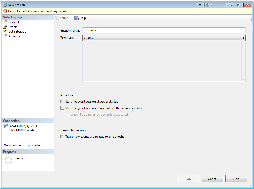
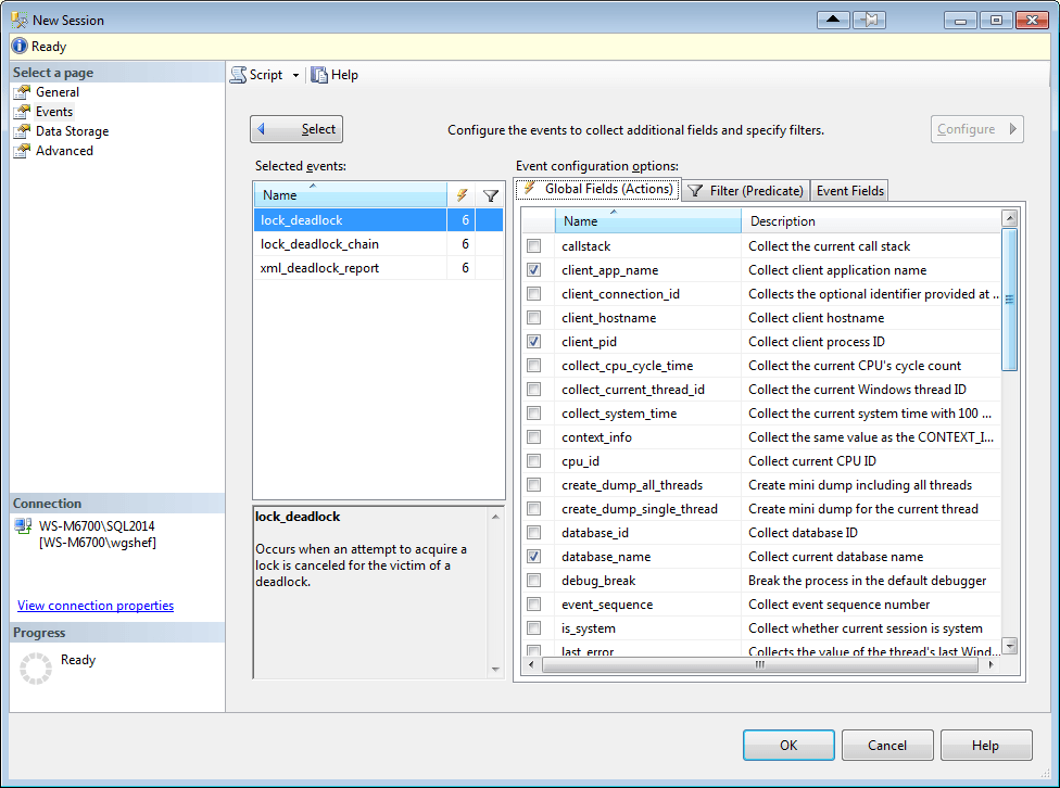
With this information, I can now jump into SSMS (2014) and use the New Session wizard to create a new XE session (Expand the Management and Extended Events nodes. Right click on Sessions and select New Session). I name the session “Deadlocks”, and click the “Events” page to select the events that I want to use.

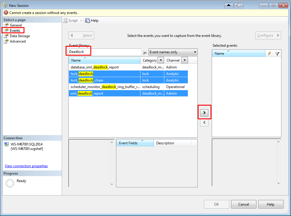
Since all of the events that I’m looking for contain “Deadlock”, I search for this and 5 events are displayed. I double-click each of the three listed above (or select them and click the “>” button) to move them to the “Selected Events” grid.

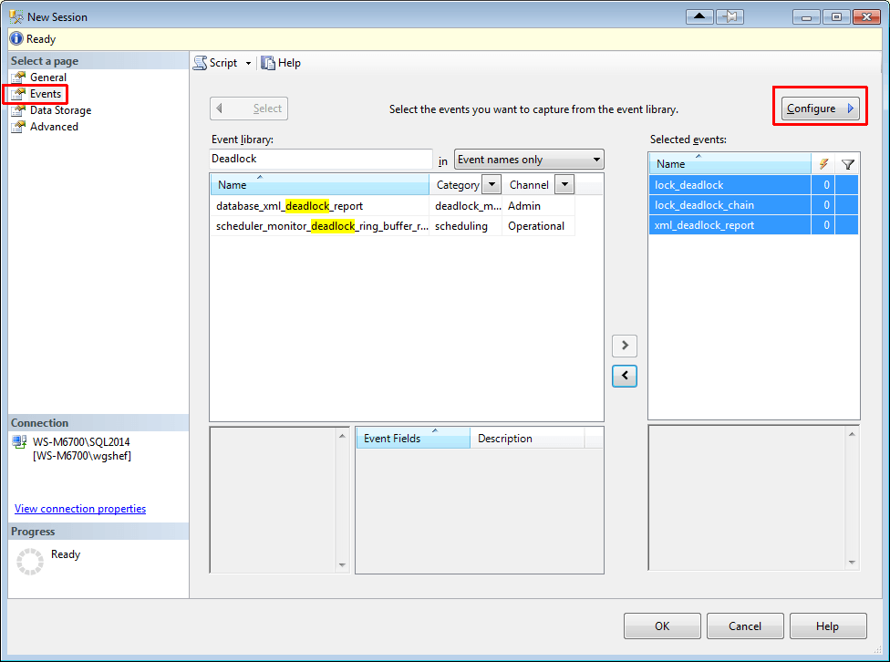
The next step is to configure the columns, so click the Configure button.

Select the lock_deadlock event, and on the “Global Fields (Actions)” tab select the client_app_name, client_pid, database_name, nt_username, server_principal_name and session_id columns.

Click on the “Event Fields” tab, and check the checkboxes for database_name and resource_description. Fields that show up in this tab with checkboxes have customizable actions, and don’t actually collect the information unless checked. Frequently this will be because these fields require an additional level of resource usage to gather this information.

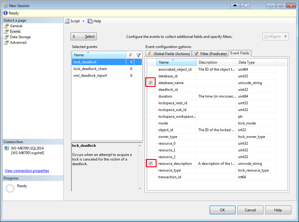
Select the lock_deadlock_chain event, and select the session_id and database_name columns on the “Global Fields (Actions)” tab. Click on the “Event Fields” tab and check the checkbox for database_name and resource_description. Finally, select the xml_deadlock_report event, and select the server_principal_name and session_id columns on the “Global Fields (Actions)” tab.

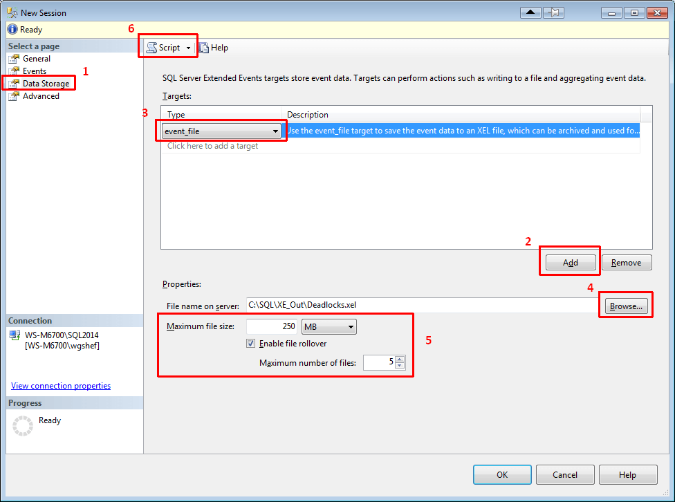
Finally, click on the Data Storage page, and add an event_file target type. The file name defaults to the name that you gave the session earlier. I set the maximum size to 250mb and 5 rollover files. If you select to script to a new query window (HIGHLY recommended), you will have a script with all of the DDL necessary to create this XE.

At this point, there are two changes that I like to make. First, I like to make my scripts so that they won’t have an error, and if the XE session already exists then one will be generated. To make it bullet-proof, I add an IF EXISTS check at the top and drop the XE session if it already exists. Secondly, I like to call xp_create_subdir to create the directory that the script points to, just in case the directory doesn’t exist. Note that xp_create_subdir will be successful if the directory already exists, so I don’t check to ensure that the directory doesn’t exist before executing this procedure.

My final XE Deadlock script looks like:

IF EXISTS (SELECT 1 FROM sys.server_event_sessions WHERE name = 'Deadlocks')
	DROP EVENT SESSION [Deadlocks] ON SERVER;
GO
EXECUTE xp_create_subdir 'C:\SQL\XE_Out';
GO
CREATE EVENT SESSION [Deadlocks]
ON SERVER
ADD EVENT sqlserver.lock_deadlock(
    SET collect_database_name=(1),collect_resource_description=(1)
	ACTION 
	(
			  sqlserver.client_app_name	-- ApplicationName from SQLTrace
			, sqlserver.client_pid	-- ClientProcessID from SQLTrace
			, sqlserver.nt_username	-- NTUserName from SQLTrace
			, sqlserver.server_principal_name	-- LoginName from SQLTrace
			, sqlserver.session_id	-- SPID from SQLTrace
	)
),
ADD EVENT sqlserver.lock_deadlock_chain(
    SET collect_database_name=(1),collect_resource_description=(1)
	ACTION 
	(
			  sqlserver.session_id	-- SPID from SQLTrace
	)
),
ADD EVENT sqlserver.xml_deadlock_report(
	ACTION 
	(
			  sqlserver.server_principal_name	-- LoginName from SQLTrace
			, sqlserver.session_id	-- SPID from SQLTrace
	)
)
ADD TARGET package0.event_file
(
	SET filename = 'C:\SQL\XE_Out\Deadlocks.xel',
		max_file_size = 250,
		max_rollover_files = 5
)
WITH (STARTUP_STATE=OFF)
;

Now that you have this XE session scripted out, it can be easily installed on multiple servers. If you encounter a deadlock problem, you can easily start the XE session and let it run to trap your deadlocks. They will be persisted to a file dedicated for the deadlocks. You can use my Deadlock Shredder script at http://bit.ly/ShredDL to read the deadlocks from the file and shred the deadlock XML into a tabular output.

Note that the default system_health XE session also captures deadlocks. I like to have a dedicated session for just deadlocks. As lightweight as XE is, sometimes it may benefit a server to turn off the system_health session. Additionally, Jonathan Kehayias has a script that will take a running trace and completely script out an XE session for it. This script can be found at https://www.sqlskills.com/blogs/jonathan/converting-sql-trace-to-extended-events-in-sql-server-2012/. Even though this script is available, I like to figure things out for myself so that I can learn what is actually going on.

Did you catch the note above where I mentioned that the default system_health XE captures deadlocks? This means that if you are still enabling trace flags 1204 and/or 1222 to capture deadlock information in your error logs, you don’t need to do that anymore. Furthermore, by using this Deadlock XE, you can have the deadlocks persisted to a file where, in combination with my Deadlock Shredder script, it will be even easier to analyze the deadlocks than trying to figure it out from the captured information in the error logs.

I hope that this post will help someone with the conversion from using SQL Profiler to using XE instead. The process for converting other traces would be the same, so it can be easily adapted. I also hope that these deadlock scripts will be helpful to you!

In my next post, I will be comparing the results of the deadlock trace and the deadlock XE session.

And Jes – thanks for hosting this month! I’m really looking forward to seeing the roundup for this month.

This post is re-published from my original post on SQL Solutions Group.

The post Weaning yourself off of SQL Profiler (Part 1) appeared first on Wayne Sheffield.

I’ve been working a lot in the Azure PowerShell area of late. One thing I wanted to be able to do is have my scripts login automatically to Azure. In many examples the cmdlet Save-AzureRmProfile was used to save your Azure credentials, then later you could use Import-AzureRmProfile to import them.

But, when I attempted to run Save-AzureRmProfile I got the error ‘Save-AzureRmProfile is not recognized as the name of a cmdlet, function, script file, or operable program’.  Huh? I checked the docs, and it does include a listing for Save-AzureRmProfile.

https://docs.microsoft.com/en-us/powershell/module/azurerm.profile/save-azurermprofile?view=azurermps-3.8.0

This is a case of the PowerShell AzureRM module getting ahead of the docs. After beating my head against the wall, I found the cmdlets had been replaced with the new noun of AzureRmContext.

To use them, first login to Azure manually. Then, use the new Save-AzureRmContext to save your information to a file.

# Setup – First login manually per previous section
Add-AzureRmAccount

# Now save your context locally (Force will overwrite if there)
$path = "C:\Azure\PS\ProfileContext.ctx’
Save-AzureRmContext -Path $path -Force

Once that’s done, from then on you can use the Import-AzureRmContext to automate the login.

# Once the above two steps are done, you can simply import
$path = ‘C:\Azure\PS\ProfileContext.ctx’
Import-AzureRmContext -Path $path

Be warned, this does present a security issue. If someone were to steal your context file, they could then login as you. You need to be sure your context file is stored in a safe location no one can get to.

Microsoft is excited to announce a new preview for the next version of SQL Server!  We disclosed a name for this next release, SQL Server 2017, today at the Microsoft Data Amp event. Community Technology Preview (CTP) 2.0 is the first production-quality preview of SQL Server 2017, and it is available on both Windows and Linux.  In this preview, we added a number of new capabilities, including the ability to run advanced analytics using Python in a parallelized and highly scalable way, the ability to store and analyze graph data, and other capabilities that help you manage SQL Server for high performance and uptime, including the Adaptive Query Processing family of intelligent database features and resumable online indexing.

In addition to all these great new features we are excited to announce a world record in the TPC-H 1TB data warehousing workload (non-clustered). The benchmark was achieved with SQL Server 2017 on Red Hat Enterprise Linux and HPE Prolliant server hardware, beating SQL Server 2016 on the same hardware handily.  This is just the first of many anticipated performance benchmarks for SQL Server 2017 on Linux and Windows, demonstrating SQL Server’s industry leading performance.  When taken in conjunction with the fact that SQL Server has had the least vulnerabilities of any major database over the last 7 years in the National Institute of Standards and Technology (NIST) vulnerability database, SQL Server 2017 on Windows and Linux is the best database for your Mission Critical application and data warehouse workloads.

You can try the preview in your choice of development and test environments now.

Key CTP 2.0 enhancements on Windows and Linux

We also added support for storing and analyzing graph data relationships. This includes full CRUD support to create nodes and edges and T-SQL query language extensions to provide multi-hop navigation using join-free pattern matching. In addition, SQL Server engine integration enables querying across SQL tables and graph data. And, you can use all of your existing SQL Server tools to work with graph data.

With resumable online index rebuild, you can resume a paused index rebuild operation from where the rebuild operation was paused rather than having to restart the operation at the beginning. Additionally, this feature rebuilds indexes using only a small amount of log space. This feature will help pick up right where you left off when an index maintenance job encounters issues, or allow you to split index rebuilds across maintenance windows.

New in SQL Server 2017, we’re adding the Adaptive Query Processing family of intelligent database features. These features automatically keep database queries running as efficiently as possible without requiring additional tuning from database administrators.  In addition to the previous capability to adjust batch mode memory grants, in CTP 2.0 Adaptive Query Processing adds the batch mode adaptive joins and interleaved execution capabilities. Interleaved execution will improve the performance of queries that reference multi-statement table valued functions by surfacing runtime row counts to the query optimizer.  Batch mode adaptive joins enables the choice of a query’s physical join algorithm to be deferred until actual query execution, improving performance based on runtime conditions.

In addition, some functionality that was previously available in SQL Server on Windows is now available on Linux for the first time. This includes:

• Additional SQL Server Agent capabilities – Use SQL Server Agent to keep replicas in synch with log shipping.
• Listener for Always On availability groups – The listener enables clients to connect to the primary replica in an availability group, monitoring availability and directing connections to the replicas.

Key CTP 2.0 enhancement to SQL Server on Windows – Python for analytics

Another new, key feature enhancement in CTP 2.0 of SQL Server 2017 is the ability to run the Python language in-database to scale and accelerate machine learning, predictive analytics and data science scripts. The new capability, called Microsoft Machine Learning Services, enables Python scripts to be run directly within the database server, or to be embedded into T-SQL scripts, where they can be easily deployed to the database as stored procedures and easily called from SQL client applications by stored procedure call. SQL Server 2017 will also extend Python’s performance and scale by providing a selection of parallelized algorithms that accelerate data transforms, statistical tests and analytics algorithms. This functionality and the ability to run R in-database and at scale are only available on Windows Server operating system at this time.

For additional detail on CTP 2.0, please visit What’s New in SQL Server 2017, Release Notes and Linux documentation.

Get SQL Server 2017 CTP 2.0 today!

Get started with the preview of SQL Server with our developer tutorials that show you how to install and use SQL Server 2017 on macOS, Docker, Windows, and Linux and quickly build an app in a programming language of your choice.

• Register to attend an Engineering Town Hall about “Security in SQL Server on Linux”
• Install on Red Hat Enterprise Linux
• Install on Ubuntu Linux
• Install on SUSE Linux Enterprise Server
• Pull and run a Linux Docker container
• Download the preview for Windows
• Create a SQL Server on Linux virtual machine in Azure
• Sign up for the Early Adoption Program (EAP) – The Early Adoption Program is designed to help customers and partners evaluate new features in SQL Server2017 and to build and deploy applications for SQL Server 2017 on Windows and Linux.

Have questions? Join the discussion of SQL Server 2017 at MSDN. If you run into an issue or would like to make a suggestion, you can let us know through Connect. We look forward to hearing from you!

This post is authored by Nagesh Pabbisetty, Partner Director of Program Management at Microsoft

Expert data scientists are adopting Advanced Analytics (AA) and Machine Learning (ML) at a rapid pace. This pace can be significantly increased when enterprise-grade AA and ML are available within environments where the customers’ data is, infusing intelligence into mission-critical applications is made much easier and, enterprises can turn to a single vendor to make the world of AA and ML synthesized and supported with the SLAs they have come to expect. At Microsoft, our mission has been to make this vision of ambient intelligence a reality for our customers. We took the first step with Microsoft R Server 9.0, and this follow on release includes significant innovations such as:

• New machine learning enhancements and inclusion of pre-trained cognitive models such as sentiment analysis & image featurizers
• SQL Server Machine Learning Services with integrated Python in Preview
• Enterprise grade operationalization with real-time scoring and dynamic scaling of VMs
• Deep customer & ISV partnerships to deliver the right solutions to customers
• A panoply of sources to help you get started with ease

You can immediately download Microsoft R Server 9.1 from MSDN and Visual Studio Dev Essentials. It comes packed with tons of value built on top of the latest open source R engine that makes R enterprise-class. Also check out R Client for Windows and R Client for Linux.

State of the Art Machine Learning

Bring Machine Learning to where your data is

With Microsoft R Server 9.0 release, we provided Machine Learning algorithms battle-tested by Microsoft as MicrosoftML package, available as a part of SQL Server R Services and Microsoft R Server  9.0 on Windows. We have now made these MicrosoftML algorithms portable and distributed to run on Linux, Windows, and the most popular distributions of Hadoop — Cloudera, Hortonworks, MapR, in addition to SQL Server 2016: Fast linear with L1 and L2 regularization, Fast boosted decision tree, Fast random forest, Logistic regression, with support for L1 and L2 regularization, GPU-accelerated Deep Neural Networks (DNNs) with convolutions, Binary classification using a One-Class Support Vector Machine. This blog demonstrates the use of Microsoft ML algorithms on Hadoop and Spark.

Pre-trained Cognitive Models

We make it easy for enterprises to infuse intelligence into their Line of Business (LOB) applications. Conventional methods require significant investments of time and effort to hand-craft Machine Learning models from scratch. Harnessing decades of work on cognitive computing in the context of Bing, Office 365 and Xbox, we are delivering the first installment of pre-trained cognitive models that accelerate time to value. Further, these models can be re-trained with your data and optimized for your business.

We now offer a Sentiment Analysis pre-trained cognitive model, using which you can assess the sentiment of an English sentence/paragraph with just a few lines of code. With the Image Featurizer pre-trained cognitive model, you can derive up to 5,000 features on a given image, and use that to compare similarity between two images. This blog shows you how to benefit from the power of image featurizers and more details of Sentiment Analysis are covered in this blog.

Combining the best of Microsoft Innovation and Open Source

We are delivering on the promise of embracing the best of open source, and pairing it with the best of Microsoft innovation. With this release, within the same R script, you can mix and match functions from RevoScaleR and Microsoft ML packages with popular open source packages like SparklyR and through it, H2O. Refer to this blog for examples on how to get the best of both worlds!

Optimized Algorithm for Pleasingly Parallel

One of the most popular advanced analytics use cases is Pleasingly Parallel where you run massively parallel computations on partitions that are grouped by one or more attributes.  These embarrassingly parallel use cases are common across industries:

• Life sciences simulations to identify the best drug for a given situation
• Portfolio analysis to identify the right investment for each portfolio
• Utilities to forecast energy consumption for each cohort
• Shipping to forecast demand for various container types

We have generalized the pattern and provided a highly performant, simple, and flexible RxExecBy() function within RevoScaleR, to address these use cases. Furthermore, this function is portable across all platforms that support Microsoft R Server — Windows, Linux, Hadoop, SQL Server. More details on how to choose the best algorithm for Pleasingly Parallel use-cases are available here.

This release also includes support for Optimized Row Columnar (ORC) file format which provides a highly efficient way to store Hive data, and distributed merge for Spark compute context, RxMerge().

Enterprise-Grade Operationalization

We recognize that easy, secure, and high-performance operationalization is essential for Tier-1 enterprises, at scale, to derive maximum value from their analytics investments. Microsoft R Server 9.1 release continues strengthening the power of operationalization. See this blog for more details.

• Real time web services: realize 10X to 100X boost in scoring performance, scoring speeds at <10ms. Currently on Windows platform; other platforms will be supported soon.
• Role Based Access Control: enables admins to control who can publish, update, delete or consume web services
• Asynchronous batch processing: speed up the scoring performance for the web services with large input data sets and long-running jobs
• Asynchronous remote execution: run scripts in background mode on a remote server, without having to wait for the job to complete
• Dynamic scaling of operationalization grid with Azure VMs: easily spin up a set of R Server VMs in Azure, configure them as a grid for operationalization, and scale it up and down based on CPU / Memory usage

SQL Server R Services

The innovations in Microsoft R Server 9.1 are available to SQL Server 2016 customers; an easy upgrade of R services in SQL Server 2016 as described in this doc and in this blog post, is all you need. The machine learning and pleasingly parallel enhancements listed in the previous section are fully supported on SQL server as well. SQL Server is the first database in the world that has in-database Machine Learning!

Real-time scoring

With R Services in SQL Server 2016, we set the industry benchmark for high throughput scoring at 1 Million predictions per second. Now, we have improved single row scoring performance significantly, up to two orders of magnitude better than earlier versions. Real-time scoring is supported on models trained using both RevoScaleR and MicrosoftML algorithms & transforms. With this release, SQL Server understands these models natively and scores inputs without the need of R interpreter and associated overhead, delivering significantly better performance.

Flexible R package management

In 9.0.1 release of Microsoft R Server we added functionality in RevoScaleR package that enables users to install, uninstall and manage packages on SQL Server without requiring administrative access to the SQL Server machine. Data scientists and other non-admin users can install packages in specific databases, user or group scope. In this release, we have added the rxSyncPackages API to ensure that the user-installed packages are not lost if the SQL Server node goes down or if the database is migrated. The list of packages and the permissions is maintained in a server table and this API ensures that the required packages are installed on the file system.

SQL Server Machine Learning Services – Python Preview

SQL Server 2016 brought you in-database analytics with SQL Server R Services. With CTP 1 of SQL Server 2017, MicrosoftML provided in-database Machine Learning.  CTP 2.0 of SQL Server 2017 brings you SQL Server Machine Learning Services that embraces both R and Python. Data Scientists can now choose from a huge collection of analytics and machine learning algorithms across R and Python communities to execute in-database and get their job done much more effectively. CTP 2.0 enables collaboration between traditional data scientists with strong R backgrounds and computer scientists with strong Python backgrounds, to deliver the best business ROI.

Additionally, the real-time scoring and flexible package management functionality listed above for SQL Server R Services is also available in the CTP2 release as part of Machine Learning services. Refer to this blog on how to get the best of both R and Python worlds!

Customer & ISV Partnerships

Engaging with Customers

“Working with Microsoft R Server for our data science needs at eToro has been a key factor in our success. The tools are appropriate for all levels of data scientist skills from beginners to seasoned professionals. Using Microsoft R Server, we were able to quickly run large scale statistical simulations in a distributed manner that ensured the robustness of our machine learning models. This partnership was instrumental in meeting our business goals and we look forward to using the continuing innovation coming out on Microsoft R Server!” — Moti Goldklang, Director of Trading Systems, eToro.

We are committed to finding more ways for our customers to connect with us, to understand how to get the most out of their investments and provide feedback to influence product direction.  We offer a variety of ways customers can engage closely with Microsoft and provide product feedback.

R Advisors: We launched R Advisors where we work with leading customers to shape our future products. Azure Advisors is an opt-in program that you can sign up on behalf of your organization.

User Voice: As a customer focus team, we are interested in listening to your feedback and to help us steer our product capability we are launching User Voice for Microsoft R today. You can partake in discussion and cast your vote on features that you’d like to see us enable. We are listening!

Authoring Tools from Microsoft and Partners

I am happy to announce that we have a number options to help you develop Microsoft R based applications, both from Microsoft and from our partners. R Tools for Visual Studio (RTVS) is now Generally Available, and brings support for Microsoft R into Visual Studio. In addition, we also have Python Tools for Visual Studio (PTVS) for your Python development. In addition, we have worked with MicroStrategy, Alteryx and KNIME, and, augmented open source Rattle, to give you more choices.

Microsoft has been contributing to the R Community to ensure that there is an open source WYSIWYG tool to do big data analytics in the community. We have enhanced the popular Rattle package to support Microsoft R Server capabilities. You can download the latest, and stay abreast with the developments here.

With Alteryx Designer 11.0, a self-service analytics workflow tool from Alteryx, business analysts and data scientists can work with Microsoft R Server and SQL Server R Services. In the words of Neil Ryan, Product Manager at Alteryx, “At Alteryx we’re acutely aware of the challenge of getting faster insights from very large datasets. When it comes to computation-intensive machine learning, it’s even more important to leverage existing hardware resources and keep the processing as close as possible to where the data lives. That’s why we’re excited about our partnership with Microsoft. By leveraging Microsoft R Server and SQL Server’s in database analytics, our customers are scaling their analytics to the size of their data through a consistent, code-free, drag and drop interface for both data preparation and modeling within SQL Server.” More details are in this blog post.

Microsoft and KNIME have partnered to bring Microsoft R capabilities to the KNIME platform. “KNIME has added the option to reach out to Microsoft R from KNIME Analytics Platform to make a scalable and enterprise ready R integration part of any KNIME workflow,” says Michael Berthold, CEO of KNIME. Here is an example of how this works and you can see it in action here.

MicroStrategy has made Microsoft R runtime accessible from MicroStrategy Desktop. “MicroStrategy is embracing Microsoft R in our analytics platform tools to bring the power of advanced analytics and machine learning to our customers. We just announced this at MicroStrategy World and you can read more about this here,” says Sandipto Banerjee, VP Data Group & Advanced Technologies, MicroStrategy.

Getting Started

The best place to get started is our comprehensive documentation site, which introduces concepts, platforms, features, code samples, and how-tos. Our vibrant blogs include R Server Blog that was  launched earlier this year on all thing R, R Tiger Team which covers deep technical insights on Microsoft R Server, and the Revolutions R Blog which highlights both Microsoft R and open-source R innovations. Together, these blogs provide a plethora of articles, tips and tricks for novices and experts alike. I welcome you to check these out and leave us your comments.

Check out the free Data Science with Microsoft SQL Server 2016 eBook that covers what’s new, installing & configuring R Services, and how to develop full applications through walkthroughs.

Want to get certified and show your mastery in data science? We have your covered via several courses at Microsoft LearnAnalytics and Microsoft Academy! We have several training partners that can help you train your teams on advanced analytics and machine learning!

Solution Templates

Check out the R Solution Templates that will walk you through how to develop a solution using Microsoft R Server, from beginning to end. In addition, with the click of a button, you can deploy these templates to an AzureVM and see the entire application in action. You can follow the links to github and use the code as a starting point for your own solution, and accelerate time to value!

In our last release, we provided a Solutions Template for Campaign Optimization using SQL Server R Services.  Now, we have added a solution template for the Azure HDInsight platform on Spark compute context.  In the words of Anindya Palit, EVP Affine Analytics, “Partnering with Microsoft allowed Affine’s extensive analytics experience in marketing to be transformed into a solution for optimizing lead generation through Campaign Optimization. We were able to quickly ramp up and build the solution utilizing the power of R Services within SQL Server.”

Hospital Length Of Stay (LOS) is the latest solution template built on SQL Server R Services. Dr. Greg Mckelvey, Head of Clinical Insights, KenSci, says “The Hospital ‘Length of Stay Prediction’ solution shows how you can build a potentially life-saving machine learning solution by leveraging the power of R within SQL Server. By predicting how long an admitted patient is likely to stay at the hospital based on clinical history, labs and vital, the solution enables doctors and nurses to better manage patient flow and coordinate post-discharge patient care.”

Azure VMs

Microsoft R Server 9.1 will be released as Azure VMs in Azure Marketplace, Data Science VMs, and on Azure HDInsight. VMs were available on CentOS 7.2 and Ubuntu 16.04. Now, we have added support for RHEL 7.2, and made all VMs available in China.

Microsoft R Client

With our current release, we are delivering Microsoft R Client on the Linux platform for the first time, in addition to Windows. R Client is available on all four popular flavors of Linux – RHEL, CentOS, Ubuntu, and SuSE.  Please check out R Client for Windows and R Client for Linux.

In Summary

I am proud of how we are making R enterprise-grade through Microsoft R portfolio of products and services, building on top of open source R in fully compatible ways. Adopting advanced analytics and machine learning requires a holistic approach that transcends technology, people and processes; we continue to deliver more handholding to ensure that enterprise users are set up for success! With the 9.1 release, you have in-database analytics and machine learning in a variety of platforms, develop powerful analytics models leveraging both open source and Microsoft innovation, deploy them at scale, and easily integrate into line-of-business systems to maximize ROI.  We invite you to get started with Microsoft R Server 9.1.

Nagesh Pabbisetty

This post was authored by Joseph Sirosh, Corporate Vice President, Microsoft Data Group

Leveraging intelligence out of the ever-increasing amounts of data can make the difference between being the next market disruptor or being relegated to the pages of history. Today at the Microsoft Data Amp online event, we will make several product announcements that can help empower every organization on the planet with data-driven intelligence. We are delivering a comprehensive data platform for developers and businesses to create the next generation of intelligent applications that drive new efficiencies, help create better products, and improve customer experiences.

I encourage you to attend the live broadcast of the Data Amp event, starting at 8 AM Pacific, where Scott Guthrie, executive VP of Cloud and Enterprise, and I will describe product innovations that integrate data and artificial intelligence (AI) to transform your applications and your business. You can stream the keynotes and access additional on-demand technical content to learn more about the announcements of the day.

Today, you’ll see three key innovation themes in our product announcements. The first is the close integration of AI functions into databases, data lakes, and the cloud to simplify the deployment of intelligent applications. The second is the use of AI within our services to enhance performance and data security. The third is flexibility—the flexibility for developers to compose multiple cloud services into various design patterns for AI, and the flexibility to leverage Windows, Linux, Python, R, Spark, Hadoop, and other open source tools in building such systems.

Hosting AI where the data lives

A novel thread of innovation you’ll see in our products is the deep integration of AI with data. In the past, a common application pattern was to create statistical and analytical models outside the database in the application layer or in specialty statistical tools, and deploy these models in custom-built production systems. That results in a lot of developer heavy lifting, and the development and deployment lifecycle can take months. Our approach dramatically simplifies the deployment of AI by bringing intelligence into existing well-engineered data platforms through a new computing model: GPU deep learning. We have taken that approach with the upcoming release of SQL Server, and deeply integrated deep learning and machine learning capabilities to support the next generation of enterprise-grade AI applications.

So today it’s my pleasure to announce the first RDBMS with built-in AI—a production-quality Community Technology Preview (CTP 2.0) of SQL Server 2017. In this preview release, we are introducing in-database support for a rich library of machine learning functions, and now for the first time Python support (in addition to R). SQL Server can also leverage NVIDIA GPU-accelerated computing through the Python/R interface to power even the most intensive deep-learning jobs on images, text, and other unstructured data. Developers can implement NVIDIA GPU-accelerated analytics and very sophisticated AI directly in the database server as stored procedures and gain orders of magnitude higher throughput. In addition, developers can use all the rich features of the database management system for concurrency, high-availability, encryption, security, and compliance to build and deploy robust enterprise-grade AI applications.

We have also released Microsoft R Server 9.1, which takes the concept of bringing intelligence to where your data lives to Hadoop and Spark, as well as SQL Server. In addition to several advanced machine learning algorithms from Microsoft, R Server 9.1 introduces pretrained neural network models for sentiment analysis and image featurization, supports SparklyR, SparkETL, and SparkSQL, and GPU for deep neural networks. We are also making model management easier with many enhancements to production deployment and operationalization. R Tools for Visual Studio provides a state-of-the-art IDE for developers to work with Microsoft R Server. An Azure Microsoft R Server VM image is also available, enabling developers to rapidly provision the server on the cloud.

In the cloud, Microsoft Cognitive Services enable you to infuse your apps with cognitive intelligence. Today I am excited to announce that the Face API, Computer Vision API, and Content Moderator are now generally available in the Azure Portal. Here are some of the different types of intelligence that cognitive services can bring to your application:

• Face API helps detect and compare human faces, organize faces into groups according to visual similarity, and identify previously tagged people in images.
• Computer Vision API gives you the tools to understand the contents of any image: It creates tags that identify objects, beings like celebrities or actions in an image, and crafts coherent sentences to describe it. You can now detect landmarks and handwriting in images. Handwriting detection remains in preview.
• Content Moderator provides machine-assisted moderation of text and images, augmented with human review tools.

Azure Data Lake Analytics (ADLA) is a breakthrough serverless analytics job service where you can easily develop and run massively parallel petabyte-scale data transformation programs that compose U-SQL, R, Python, and .NET. With no infrastructure to manage, you can process data on demand, scale instantly, and pay per job only. Furthermore, we’ve incorporated the technology that sits behind the Cognitive Services inside U-SQL directly as functions. Now you can process massive unstructured data, such as text/images, extract sentiment, age, and other cognitive features using Azure Data Lake, and query/analyze these by content. This enables what I call “Big Cognition—it’s not just extracting one piece of cognitive information at a time, and not just about understanding an emotion or whether there’s an object in an individual image, but rather it’s about integrating all the extracted cognitive data with other types of data, so you can perform powerful joins, analytics, and integrated AI.

Azure Data Lake Store (ADLS) is a no-limit cloud HDFS storage system that works with ADLA and other big data services for petabyte-scale data. We are announcing the general availability of Azure Data Lake Analytics and Azure Data Lake Store in the Azure North Europe region.

Yet another powerful integration of data and AI is the seamless integration of DocumentDB with Spark to enable machine learning and advanced analytics on top of globally distributed data. To recap, DocumentDB is a unique, globally distributed, limitless NoSQL database service in Azure designed for mission-critical applications. Designed as such from the ground up, it allows customers to distribute their data across any number of Azure regions worldwide, guarantees low read and write latencies, and offers comprehensive SLAs for data-loss, latency, availability, consistency, and throughput. You can use it as either your primary operational database or as an automatically indexed, virtually infinite data lake. The Spark connector understands the physical structure of DocumentDB store (indexing and partitioning) and enables computation pushdown for efficient processing. This service can significantly simplify the process of building distributed and intelligent applications at global scale.

I’m also excited to announce the general availability of Azure Analysis Services. Built on the proven business intelligence (BI) engine in Microsoft SQL Server Analysis Services, it delivers enterprise-grade BI semantic modeling capabilities with the scale, flexibility, and management benefits of the cloud. Azure Analysis Services helps you integrate data from a variety of sources—for example, Azure Data Lake, Azure SQL DW, and a variety of databases on-premises and in the cloud—and transform them into actionable insights. It speeds time to delivery of your BI projects by removing the barrier of procuring and managing infrastructure. And by leveraging the BI skills, tools, and data your team has today, you can get more from the investments you’ve already made.

Stepping up performance and security

Performance and security are central to databases. SQL Server continues to lead in database performance benchmarks, and in every release we make significant improvements. SQL Server 2016 on Windows Server 2016 holds a number of records on the Transaction Processing Performance Council (TPC) benchmarks for operational and analytical workload performance, and SQL Server 2017 does even better. I’m also proud to announce that the upcoming version of SQL Server will run just as fast on Linux as on Windows, as you’ll see in the newly published 1TB TPC-H benchmark world record nonclustered data warehouse performance achieved with SQL Server 2017 on Red Hat Enterprise Linux and HPE ProLiant hardware.

SQL Server 2017 will also bring breakthrough performance, scale, and security features to data warehousing. With up to 100x faster analytical queries using in-memory Columnstores, PolyBase for single T-SQL querying across relational and Hadoop systems, capability to scale to hundreds of terabytes of data, modern reporting, plus mobile BI and more, it provides a powerful integrated data platform for all your enterprise analytics needs.

In the cloud, Azure SQL Database is bringing intelligence to securing your data and increasing database performance. Threat Detection in Azure SQL Database works around the clock, using machine learning to detect anomalous database activities indicating unusual and potentially harmful attempts to access or exploit databases. Simply turning on Threat Detection helps customers make databases resilient to the possibility of intrusion. Other features of Azure SQL Database such as auto-performance tuning automatically implement, tune, and validate performance to guarantee the most optimal query performance. Together, our intelligent database management features help make your database more secure and faster automatically, freeing up scarce DBA capacity for more strategic work.

Simple, flexible multiservice AI solutions in the cloud

We are very committed to simplifying the development of AI systems. Cortana Intelligence is a collection of fully managed big data and analytics services that can be composed together to build sophisticated enterprise-grade AI and analytics applications on Azure. Today we are announcing Cortana Intelligence solution templates that make it easy to compose services and implement common design patterns. These solutions templates have been built on best practice designs motivated by real-world customer implementations done by our engineering team, and include Personalized Offers (for example, for retail applications), Quality Assurance (for example, for manufacturing applications), and Demand Forecasting. These templates accelerate your time to value for an intelligent solution, allowing you to deploy a complex architecture within minutes, instead of days. The templates are flexible and scalable by design. You can customize them for your specific needs, and they’re backed by a rich partner ecosystem trained on the architecture and data models. Get started today by going to the Azure gallery for Cortana Intelligence solutions.

Also, AppSource is a single destination to discover and seamlessly try business apps built by partners and verified by Microsoft. Partners like KenSci have already begun to showcase their intelligent solutions targeting business decision-makers in AppSource. Now partners can submit Cortana Intelligence apps at AppSource “List an app” page.

Cross-platform and open source flexibility

Whether on-premises or in the cloud, cross-platform compatibility is increasingly important in our customers’ diverse and rapidly changing data estates. SQL Server 2017 will be the first version of SQL Server compatible with Windows, Linux, and Linux-based container images for Docker. In addition to running on Windows Server, the new version will also run on Red Hat Enterprise Linux, SUSE Enterprise Linux Server, and Ubuntu. It can also run inside Docker containers on Linux or Mac, which can help your developers spend more time developing and less on DevOps.

Getting started

It has never been easier to get started with the latest advances in the intelligent data platform. We invite you to join us to learn more about SQL Server 2017 on Windows, Linux, and in Linux-based container images for Docker; Cognitive Services for smart, flexible APIs for AI; scalable data transformation and intelligence from Azure Data Lake Store and Azure Data Lake Analytics; the Azure SQL Database approach to proactive threat detection and intelligent database tuning; new solution templates from Cortana Intelligence; and precalibrated models for Linux, Hadoop, Spark, and Teradata in R Server 9.1.

Join our Data Amp event to learn more! You can go now to the Microsoft Data Amp online event for live coverage starting at 8 AM Pacific on April 19. You’ll also be able to stream the keynotes and watch additional on-demand technical content after the event ends. I look forward to your participation in this exciting journey of infusing intelligence and AI into every software application.

We are excited to share the preview release of in-database analytics and machine learning with Python in SQL Server. Python is one of the most popular languages for data science and has a rich ecosystem of powerful libraries.

Starting with the CTP 2.0 release of SQL Server 2017, you can now bring Python-based intelligence to your data in SQL Server.

The addition of Python builds on the foundation laid for R Services in SQL Server 2016 and extends that mechanism to include Python support for in-database analytics and machine learning. We are renaming R Services to Machine Learning Services, and R and Python are two options under this feature.

The Python integration in SQL Server provides several advantages:

• Elimination of data movement: You no longer need to move data from the database to your Python application or model. Instead, you can build Python applications in the database. This eliminates barriers of security, compliance, governance, integrity, and a host of similar issues related to moving vast amounts of data around. This new capability brings Python to the data and runs code inside secure SQL Server using the proven extensibility mechanism built in SQL Server 2016.
• Easy deployment: Once you have the Python model ready, deploying it in production is now as easy as embedding it in a T-SQL script, and then any SQL client application can take advantage of Python-based models and intelligence by a simple stored procedure call.
• Enterprise-grade performance and scale: You can use SQL Server’s advanced capabilities like in-memory table and column store indexes with the high-performance scalable APIs in RevoScalePy package. RevoScalePy is modeled after RevoScaleR package in SQL Server R Services. Using these with the latest innovations in the open source Python world allows you to bring unparalleled selection, performance, and scale to your SQL Python applications.
• Rich extensibility: You can install and run any of the latest open source Python packages in SQL Server to build deep learning and AI applications on huge amounts of data in SQL Server. Installing a Python package in SQL Server is as simple as installing a Python package on your local machine.
• Wide availability at no additional costs: Python integration is available in all editions of SQL Server 2017, including the Express edition.

Data scientists, application developers, and database administrators can all benefit from this new capability.

• Data scientists can build models using the full datasets on the SQL Server instead of moving data to your IDE or being forced to work with samples of data. Working from your Python IDE, you can execute Python code that runs in SQL Server on the data in SQL Server and get the results in your IDE. You are no longer dependent on application developers to deploy your models for production use, which often involves translating models and scripts to a different application language. These models can be deployed to production easily by embedding them in T-SQL stored procedures. You can use any open source Python package for machine learning in SQL Server. The usage pattern is identical to the now popular SQL Server R Services.
• Application developers can take advantage of Python-based models by simply making a stored procedure call that has Python script embedded in it. You don’t need a deep understanding of the inner workings of the Python models, or have to translate it to a line of business language in close coordination with data scientists to consume it. You can even leverage both R and Python models in the same application—they are both stored procedure calls.
• Database administrators can enable Python-based applications and set up policies to govern how Python runtime behaves on SQL Server. You can manage, secure, and govern the Python runtime to control how the critical system resources on the database machine are used. Security is ensured by mechanisms like process isolation, limited system privileges for Python jobs, and firewall rules for network access.

The standard open source CPython interpreter (version 3.5) and some Python packages commonly used for data science are downloaded and installed during SQL Server setup if you choose the Python option in the feature tree.

Currently, a subset of packages from the popular Anaconda distribution is included along with Microsoft’s RevoScalePy package. The set of packages available for download will evolve as we move toward general availability of this feature. Users can easily install any additional open source Python package, including the modern deep learning packages like Cognitive Toolkit and TensorFlow to run in SQL Server. Taking advantage of these packages, you can build and deploy GPU-powered deep learning database applications.

Currently, Python support is in “preview” state for SQL Server 2017 on Windows only.

We are very excited about the possibilities this integration opens up for building intelligent database applications. Please watch the Python based machine learning in SQL Server presentation and Joseph Sirosh Keynote at Microsoft Data Amp 2017 event for demos and additional information. We encourage you to install SQL Server 2017. Please share your feedback with us as we work toward general availability of this technology.

Thank you!

Sumit Kumar, Senior Program Manager, SQL Server Machine Learning Services

Nagesh Pabbisetty, Director of Program Management, Microsoft R Server and Machine Learning

Hello

I have just gathered all sessions (deep dive ones) that you might have seen live on 4/19. Look how many sessions are there!!!!

• Security on Linux with Tommy Mullaney - http://bit.ly/2onopRi
• Build globally-scaled mobile apps in minutes with Kirill Gavrylyuk -  http://bit.ly/2oQssXl
• What's new with Azure Machine Learning with Ted Way - http://bit.ly/2pDnahz
• Building an intelligent Bot with Paul Stubbs - http://bit.ly/2pDTHUX
• Transform healthcare with advanced analytics solutions with Todd Bergeson - http://bit.ly/2oWVHd3
• Adding intelligence to your applications using big data at scale with Saveen Reddy - http://bit.ly/2pSWLvQ
• SQL Server 2017: HA and DR on Linux with Mihaela Blendea - http://bit.ly/2oWZhUu
• SQL Server Virtual Machines: Getting Started with Luis Vargas - http://bit.ly/2pDUJAo
• Developing Xamarin based data-driven intelligent applications using Azure Data Services (ADS) with Tara Shankar Jana - http://bit.ly/2oWIeC0
• Enterprise-ready Data Warehousing in the Cloud with Josh Caplan - http://bit.ly/2o5j6K5
• Developing applications with SQL Server 2017 (Linux), Entity Framework, DevOps and Azure with Tara Shankar Jana - http://bit.ly/2phlCgk
• Python based machine learning in SQL Server with Sumit Kumar and Vijay Jayaseelan - http://bit.ly/2pDTTmT
• SQL Server 2017: Building applications using graph data with Shreya Verma - http://bit.ly/2pSVpku
• SQL Server 2017: What's New in the Database Engine? with Travis Wright - http://bit.ly/2o5gPi4
• Overview of Microsoft Machine Language R package with Gleb Krivosheev and Yunling Wang - http://bit.ly/2oQKc4D
• Get started developing apps with SQL Server 2017 running on Linux with David Salgado - http://bit.ly/2oQBm6U
• Accelerate your journey to advanced analytics solutions with Kuber Sharma - http://bit.ly/2o5l4Kp
• Get started with Azure Analysis Services with Josh Caplan - http://bit.ly/2oMZb1d
• What's new in R Server 9.1 and SQL R Services with Nagesh Pabbisetty - http://bit.ly/2pDGTR3
• Transform retail with Advanced Analytics solutions with Esther Christoffersen - http://bit.ly/2ot8Fez
• Big data that is easy and productive with Azure Data Lake with Saveen Reddy - http://bit.ly/2otlwgK
• Transform traditional data warehouse with cloud and big data with Oliver Chiu - http://bit.ly/2phgmcC
• SQL Server 2017: Adaptive query processing with Joe Sack - http://bit.ly/2otjfSF
• Make your apps faster and more secure in SQL Server 2016 SP1 Standard and Express Edition with Travis Wright - http://bit.ly/2o5mMeT
• The app developer's managed cloud database (overview) with Lindsey Allen - http://bit.ly/2o5ke0p
• Transform manufacturing with Advanced Analytics solutions with Colin Masson - http://bit.ly/2oMA4vk
• SQL Server 2017: BI enhancements with Christian Wade - http://bit.ly/2oo0Tne
• Breakthrough performance with SQL Server for data warehousing (new RAs) with Jamie Reding - http://bit.ly/2phsJWc
• Enable applications to beat the speed of light with planet-scale DocumentDB with Sayam Nair - http://bit.ly/2phxBuw
• Transforming customer care with Business Analytics and AI with Seayoung Rhee and Giampaolo Battaglia - http://bit.ly/2ot9hkm
• Deploy an intelligent solution with solution templates with Sachin Chouksey - http://bit.ly/2oMKOdj
• Build intelligence into your apps with SQL Server 2016 with Nellie Gustafsson - http://bit.ly/2oQRdCI
• What’s new with Microsoft Cognitive Services with Anna Roth - http://bit.ly/2phpL4a
• Top reasons to run SQL Server on Azure VM with Luis Vargas and Wynn Johnson - http://bit.ly/2phgc53
• SQL Server 2017 Scale Out with Mihaela Blendea and Travis Wright - http://bit.ly/2otoqlX
• Modernize your database infrastructure with DBaaS in Azure with Lindsey Allen and Murat Ozturan - http://bit.ly/2pDKfDG
• Unleash your data from non-Microsoft data platforms with Murat Ozturan - http://bit.ly/2oWU1ju

In case you missed the event and would like to – you can find all the sessions here: http://bit.ly/2pT1tcO

Cheers

Damian

Trusting big data requires understanding its data lineage. Without data lineage, big data becomes synonymous with the last phrase in a game of telephone. The original data from the first person (e.g., “a guppy swims in a shark tank”) changes to something completely different when it ends with the last person (e.g., “The puppy that […]

The post Data Lineage Demystified appeared first on DATAVERSITY.

by Angela Guess A recent press release states, “Scality, world leader in object and cloud storage, today announced immediate availability of a new open-source Scality S3 Server release, under the Apache 2.0 license, with support for high availability and multiple cloud data backends. Scality S3 Server’s extensive multi-cloud support now includes AWS S3, In-memory, Scality […]

The post Scality Accelerates Multi-Cloud Adoption with New Open-Source Release appeared first on DATAVERSITY.

by Angela Guess A recent press release reports, “IBM today introduced new cognitive capabilities for IBM Watson Marketing Insights, a cloud-based offering that continuously examines customer behavior and learns how it may impact the success of the business. With these insights marketing teams can take action to launch targeted campaigns designed to turn all customers […]

The post IBM Puts Watson into the Hands of Marketing Professionals appeared first on DATAVERSITY.

The latest release of Is It SQL now shows missing backups.

Backups

The top section gives you a summary of all servers with missing backups and the bottom section lists each individual database that doesn't have a good backup. Right now a "good" full backup is defined as being a full or differential within the last thirty-six hours. Further, a database in FULL recovery model expects a log backup within the last ninety minutes.

The last backup query can be a little expensive so it only polls backups every five minutes. If you have more than a million rows of backup history it doesn't poll that server's backups at all. It will include a message indicating this.

There's a simple text file you can edit to exclude servers and databases from expecting to be backed up. If you have multiple connections to a server (availability group name and node name) it will still only appear once.

And if you're reading this, welcome to the new blog. That means the RSS feed updated properly. Or at least you found it some other way.

More Concurrent Polling

The number of concurrent servers it will poll has been increased to eight. This seems to work well so far. I originally increased this to handle slow backup queries but finally gave in and just fixed the backup queries. But eight concurrent pollers seems to work well so far.

The "Infographic"

I really want to add a cool infographic showing a summary of your environment. I've got the numbers but not the graphic part. So for now I'm calling it a summary.

I'm surprised at just how many databases there are in some the environments I monitor with this. It's also been interesting to watch the total IOPS across all servers in near-real time. As you can see, my little development box isn't very interesting.

Miscellaneous

• Various wait group names have been cleaned up. Mostly with regard to SQL Server 2016 and availability groups.

• If sys.dm_exec_requests shows a percent complete then so does Is It SQL. If you hover over the duration on the Active Sessions page for a server it will show the start time and percent complete. I mostly use this to obsess over backups and restores.

SQL Server is trusted by many customers for enterprise-grade, mission-critical workloads that store and process large volumes of data. Technologies like in-memory OLTP and columnstore have also helped our customers to improve application performance many times over. But when it comes to hierarchical data with complex relationships or data that share multiple relationships, users might find themselves struggling with a good schema design to represent all the entities and relationships, and writing optimal queries to analyze complex data and relationships between the tables. SQL Server uses foreign keys and joins to handle relationships between entities or tables. Foreign keys only represent one-to-many relationships and hence, to model many-to-many relationships, a common approach is to introduce a table that holds such relationships. For example, Student and Course in a school share a many-to-many relationship; a Student takes multiple Courses and a Course is taken by multiple Students. To represent this kind of relationship one can create an “Attends” table to hold information about all the Courses a Student is taking. The “Attends” table can then store some extra information like the dates when a given Student took this Course, etc.

Over time applications tend to evolve and get more complex. For example, a Student can start “Volunteering” in a Course or start mentoring “Mentoring” others. This will add new types of relationships to the database. With this type of approach, it is not always easy to modify existing tables to accommodate evolving relationships. To analyze data connected by means of foreign keys or multiple junction tables involves writing complex queries with joins across multiple tables, and this is no trivial task. The queries can quickly get complex, resulting in complex execution plans and degraded query performance over time.

We live in an era of big data and connected information; people, machines, devices, businesses across the continents are connected to each other more than ever before. Analyzing connected information is becoming critical for businesses to achieve operational agility. Users are finding it easier to model data and complex relationships with the help of graph databases. Native graph databases have risen in popularity, being used for social networks, transportation networks, logistics, and much more. Graph database scenarios can easily be found across several business disciplines, including supply chain management, computer or telecommunication networks, detecting fraud attacks, and recommendation engines.

At Microsoft, we believe that there should be no need for our customers to turn to a new system just to meet their new or evolving graph database requirements. SQL Server is already trusted by millions of customers for mission-critical workloads, and with graph extensions in SQL Server 2017, customers get the best of both relational and graph databases in a single product, including the ability to query across all data using a single platform. Users can also benefit from other cutting-edge technologies already available in SQL Server, such as columnstore indexes, advanced analytics using SQL Server R Services, high availability, and more.

Graph extensions available in SQL Server 2017

A graph schema or database in SQL Server is a collection of node and edge tables. A node represents an entity—for example, a person or an organization—and an edge represents a relationship between the two nodes it connects. Figure 1 shows the architecture of a graph database in SQL Server.

Figure 1: SQL graph database architecture

Create graph objects

With the help of T-SQL extensions to DDL, users can create node or edge tables. Both nodes and edges can have properties associated to them. Users can model many-to-many relationships using edge tables. A single edge type can connect multiple type of nodes with each other, in contrast to foreign keys in relational tables. Figure 2 shows how a node and edge table are stored internally in the database. Since nodes and edges are stored as tables, most of the operations supported on tables are available on node or edge tables, too.

Figure 2: Person Node and Friends Edge table.

The CREATE TABLE syntax guide shows the supported syntax for creation of node and edge tables.

Query language extensions

To help search a pattern or traverse through the graph, a new MATCH clause is introduced that uses ASCII-art syntax for pattern matching and navigation. For example, consider the Person and Friends node tables shown in Figure 2; the following query will return friends of “John”:

SELECT Person2.Name
FROM Person Person1, Friends, Person Person2
WHERE MATCH(Person1-(Friends)->Person2)
AND Person1.Name = ‘John’;

The MATCH clause is taking a search pattern as input. This pattern traverses the graph from one node to another via an edge. Edges appear inside parentheses and nodes appear at the ends of the arrow. Please refer to MATCH syntax guide to find out more ways in which MATCH can be used.

Fully integrated in SQL Server engine

Graph extensions are fully integrated in the SQL Server engine. Node and edge tables are just new types of tables in the database. The same storage engine, metadata, query processor, etc., is used to store and query graph data. All security and compliance features are also supported. Other cutting-edge technologies like columnstore, ML using R Services, HA, and more can also be combined with graph capabilities to achieve more. Since graphs are fully integrated in the engine, users can query across their relational and graph data in a single system.

Tooling and ecosystem

Users benefit from the existing tools and ecosystem that SQL Server offers. Tools like backup and restore, import and export, BCP, and SSMS “just work” out of the box.

FAQs

How can I ingest unstructured data?

Since we are storing data in tables, users must know the schema at the time of creation. Users can always add new types of nodes or edges to their schema. But if they want to modify an existing node or edge table, they can use ALTER TABLE to add or delete attributes. If you expect any unknown attributes in your schema, you could either use sparse columns or create a column to hold JSON strings and use that as a placeholder for unknown attributes.

Do you maintain an adjacency list for faster lookups?

No. We are not maintaining an adjacency list on every node; instead we are storing edge data in tables. Because it is a relational database, storing data in the form of tables was a more natural choice for us. In native-directed graph databases with an adjacency list, you can only traverse in one direction. If you need to traverse in the reverse direction, you need to maintain an adjacency list at the remote node too. Also, with adjacency lists, in a big graph for a large query that spawns across your graph, you are essentially always doing a nested loop lookup: for every node, find all the edges, from there find all the connected nodes and edges, and so on.

Storing edge data in a separate table allows us to benefit from the query optimizer, which can pick the optimal join strategy for large queries. Depending on the complexity of query and data statistics, the optimizer can pick a nested loop join, hash join, or other join strategies — as opposed to always using nested loop join, as in the case of an adjacency list. Each edge table has two implicit columns, $from_id and $to_id, which store information about the nodes that it connects. For OLTP scenarios, we recommend that users create indexes on these columns ($from_id, $to_id) for faster lookups in the direction of the edge. If your application needs to perform traversals in reverse direction of an edge, you can create an index on ($to_id, $from_id).

Is the new MATCH syntax supported on relational tables?

No. MATCH clause works only on graph node and edge tables.

Can I alter an existing table into a node or edge table?

No. In the first release, ALTER TABLE to convert an existing relational table into a node or edge table is not supported. Users can create a node table and use INSERT INTO … SELECT FROM to populate data into the node table. To populate an edge table from an existing table, proper $from_id and $to_id values must be obtained from the node tables.

What are some table operations that are not supported on node or edge tables?

In the first release, node or edge tables cannot be created as memory-optimized, system-versioned, or temporary tables. Stretching or creating a node or edge table as external table (PolyBase) is also not supported in this release.

How do I find a node connected to me, arbitrary number of hops away, in my graph?

The ability to recurse through a combination of nodes and edges, an arbitrary number of times, is called transitive closure. For example, find all the people connected to me through three levels of indirections or find the employee chain for a given employee in an organization. Transitive closure is not supported in the first release. A recursive CTE or a T-SQL loop may be used to work around these types of queries.

How do I find ANY Node connected to me in my graph?

The ability to find any type of node connected to a given node in a graph is called polymorphism. SQL graph does not support polymorphism in the first release. A possible workaround is to write queries with UNION clause over a known set of node and edge types. However, this workaround is good for a small set of node and edge types.

Are there special graph analytics functions introduced?

Some graph databases provide dedicated graph analytical functions like “shortest path” or “page rank.” SQL Graph does not provide any such functions in this release. Again, T-SQL loops and temp tables may be used to write a workaround for these scenarios.

Thank you for reading this post! We are excited to announce the first version of graph extensions to SQL Server. To learn more, see this article on Graph processing with SQL Server 2017. Stay tuned for more blog posts and updates on SQL graph database!

Try SQL Server 2017

Get started with the preview of SQL Server 2017 on macOS, Docker, Windows, and Linux using these links:

• Install on Red Hat Enterprise Linux
• Install on Ubuntu Linux
• Install on SUSE Linux Enterprise Server
• Pull and run a Linux Docker container
• Download the preview for Windows

We are delighted to announce that Resumable Online Index Rebuild is now available for public preview in the SQL Server vNext 2017 CTP 2.0 release. With this feature, you can resume a paused index rebuild operation from where the rebuild operation was paused rather than having to restart the operation at the beginning. In addition, this feature rebuilds indexes using only a small amount of log space. You can use the new feature in the following scenarios:

• Resume an index rebuild operation after an index rebuild failure, such as after a database failover or after running out of disk space. There is no need to restart the operation from the beginning. This can save a significant amount of time when rebuilding indexes for large tables.
• Pause an ongoing index rebuild operation and resume it later. For example, you may need to temporarily free up system resources to execute a high priority task or you may have a single maintenance window that is too short to complete the operation for a large index. Instead of aborting the index rebuild process, you can pause the index rebuild operation and resume it later without losing prior progress.
• Rebuild large indexes without using a lot of log space and have a long-running transaction that blocks other maintenance activities. This helps log truncation and avoid out-of-log errors that are possible for long-running index rebuild operations.

Read the articles: The following articles provide detailed and updated information about this feature:

• Guidelines for Online Index Operations
• ALTER INDEX (Transact-SQL)
• sys.index_resumable_operations

Public preview information: For public preview communication on this topic, please contact the ResumableIDXPreview@microsoft.com alias.

To try SQL Server 2017: Get started with the preview of SQL Server 2017 on macOS, Docker, Windows, and Linux.

• Install on Red Hat Enterprise Linux
• Install on Ubuntu Linux
• Install on SUSE Linux Enterprise Server
• Pull and run a Linux Docker container
• Download the preview for Windows

Click to learn more about video blogger Stefan Groschupf. Introducing the Big Data & Brews video blog series presented by Stefan Groschupf, Founder of Datameer. The series will touch on hot topics within the business of  Big Data, Analytics, Internet of Things, Cloud Computing, Machine Learning, Modern BI, NoSQL and Next Generation Technologies. In today’s video blog Stefan Groschupf […]

The post Data Security in the Cloud appeared first on DATAVERSITY.

Authored by Arvind Shyamsundar and Shreya Verma

Reviewed by Dimitri Furman, Joe Sack, Sanjay Mishra, Denzil Ribeiro, Mike Weiner, Rajesh Setlem

Graphs are a very common way to represent networks and relationships between objects. Historically, it is not easy to represent such data structures in relational databases like SQL Server and Azure SQL DB. To address this requirement, in November 2016 (through a private preview program for a set of early adopter customers) we introduced extensions to which allow us to natively store and query graphs inside the database on Azure SQL DB.

We recently made these features publicly available as part of the SQL Server 2017 CTP 2.0 release (note that the feature is still in private preview for Azure SQL DB at this time). Please review this related blog post for an overview of the feature. In our blog post we look at a typical use case for graph data in SQL Server and Azure SQL DB.

Scenario

A common scenario we’ve seen with our early adopter customers is their interest to use graph technology to implement ‘recommendation systems’. For this walkthrough, imagine we have to implement a recommendation system for songs. Specifically, let’s imagine a scenario where there’s a user who likes Lady Gaga’s song ‘Just Dance‘. Now, our objective is to implement a recommendation system which will suggest songs which are similar to ‘Just Dance’. So, how do we get started? First, we need data!

What data can we use?

Many approaches to implementing recommendation systems involve using two distinct sets of data: one which contains users, and the other which contains details of the entities that those users are related to.

• In retail scenarios, these would be the products purchased by the user.
• In our current scenario, these are the songs which those users listened to.

It so happens that there is an amazing source of such data for songs and ‘user tastes’ (which songs did each user listen to) available online. This dataset is called the Million Song Dataset (MSD), and while it has a lot of other information, the specific subset of data that is of immediate interest to us is summarized below:

• The list of all the songs is contained in a delimited file available  here. There are a million songs in this dataset.
• On the MSD website there is a link to another dataset called the  ‘User Taste Profile’ data which contains (anonymized) user listening profiles and that is available here. There are a million unique users, and a total of 48 million ‘relationships’ (each corresponding to a row in this file) in this dataset.

What algorithm?

Now that we know what data is available to us, let’s think about the algorithm to be used. A standard approach called collaborative filtering can be used in conjunction with our graph data. Presented below is a simplified graphical representation of the algorithm that we will use.

As you can see from the animation, the algorithm is quite simple:

• First, we identify the user and ‘current’ song to start with (red line)
• Next, we identify the other users who have also listened to this song (green line)
• Then we find the other songs which those other users have also listened to (blue, dotted line)
• Finally, we direct the current user to the top songs from those other songs, prioritized by the number of times they were listened to (this is represented by the thick violet line.)

The algorithm above is quite simple, but as you will see it is quite effective in meeting our requirement. Now, let’s see how to actually implement this in SQL Server 2017.

Implementation

To begin, we recommend that you quickly review this feature overview video as well as the official documentation links for more details on the new functionality:

• An overview of Graph data in SQL Server
• Architecture details for Graph data in SQL Server
• The official sample for Graph data in SQL Server

Once you have the background, it’s easy to understand how to represent the scenario as ‘graph tables’ in SQL Server 2017. We will create two ‘node’ tables – one for the users and one for the songs. We will then ‘connect’ these two node tables with an ‘edge’ table. Here’s a quick visual summary of what we will be doing:

Importing the data

Now, let’s get to the nuts and bolts! The first step is to declare tables into which we will insert the source data. These ‘staging’ tables are ‘regular’ tables and have no ‘graph’ attributes. Here are the scripts for this:

The next step is to use the OPENROWSET BULK functionality to rapidly ingest the text files into their staging tables in SQL Server. Here are the scripts for this:

Constructing the graph

Once we have the raw data in staging tables, we can then ‘convert’ them into their Graph equivalents. Here are the table definitions; note the usage of AS NODE and AS EDGE to define the tables involved in the graph:

To actually ‘convert’ the data, we use INSERT…SELECT statements as shown below:

Querying the graph

Now that we have all the data in the ‘graph’ form, we can proceed to use the new MATCH function to express our query over the set of nodes and edges. The query below finds songs that are similar to Lady Gaga’s song called ‘Just Dance’!

Optimizing performance

The above query performs relatively quickly (in around 3 seconds on a laptop with an i7 processor). Consider that this query has to deal with a million users, a million songs and 48 million relationships between those entities. Most of the cost is taken by the time to scan through the tables, one row at a time and then match them using hash joins, as you can visualize by looking at the execution plan:

While 3 seconds is not bad, can we make this even faster? The good news is that in SQL Server 2017 CTP 2.0, graph tables support clustered columnstore indexes. While the compression offered is definitely going to help reduce I/O, the bigger benefit is that queries on these tables leverage the ‘batch-mode’ execution which allows much faster execution of queries. This is really useful for us given that the above query is doing large aggregations (GROUP BY). Let’s proceed to create these clustered columnstore indexes:

Once we create these indexes, the performance actually improves substantially and reduces the query execution time to half a second, which is 6x faster than before. That’s really impressive considering the sheer amount of data that the query needs to look at to arrive at the result!
Let’s take a minute to look at the new execution plan. Observe the ‘Batch mode’ execution highlighted below:

The other interesting thing to note is the new adaptive join type highlighted above. This is great to see – queries on graph data benefit with these new query processing improvements inside SQL Server 2107!

Let’s summarize the ‘before’ and ‘after’ states:

In summary, having graph data inside SQL Server allows database administrators and developers to leverage the familiar, mature and robust query processing capabilities within SQL Server. This is crucial to reducing the learning curve and likely complexity associated with using other technologies to store and query graph data.

Visualizing graphs

While we can use external applications and tools like PowerBI to visualize graphs, the ‘icing on the cake’ is the fact that we can use R Services in SQL Server to visualize graph data. With an open-source R package called ‘igraph’ we can visualize graphs relatively easily and render them to standard image formats like PNG. Here is a code snippet showing you how that can be done:

Here’s a section of the visualization (refer the comments in the above script to understand what the visualization represents) generated. While it is quite basic, but as you can see it is functionally very useful:

Conclusion

The support for graph data in SQL Server 2017 is an exciting new development and opens up doors to a new category of workloads which can leverage this functionality. It is one more step in bringing algorithms and intelligence closer to where the data resides.

Recommendation systems (such as the simple example presented here), fraud detection systems, content and asset management and many other scenarios can also benefit from the integration that graph data in SQL Server 2017 offers. The support for graph data in the database will be also be publicly available for Azure SQL DB in due course of time.

The complete code for this walkthrough is available here. Please use the Comments section below to ask questions and provide your feedback. We are eager to hear from you!

Citations

Thierry Bertin-Mahieux, Daniel P.W. Ellis, Brian Whitman, and Paul Lamere. The Million Song Dataset. In Proceedings of the 12th International Society for Music Information Retrieval Conference (ISMIR 2011), 2011.

The Echo Nest Taste profile subset, the official user data collection for the Million Song Dataset, available at: http://labrosa.ee.columbia.edu/millionsong/tasteprofile

• Data security concerning the application network
• Database
• Internet of things
• Security on the cloud
• Digital identity protection
  

RWDG Slides: Governing Data Governance and Master Metadata from DATAVERSITY To view the On Demand recording, click HERE>> About the Webinar Data Governance and Master Metadata are types of metadata collected about the accountability for master data across the organization. These are types of data about data – but better still they are metadata that […]

The post RWDG Slides: Governing Data Governance and Master Metadata appeared first on DATAVERSITY.