Mrdenny

Read committed is the second weakest of the four isolation levels defined by the SQL standard. Nevertheless, it is the default isolation level for many database engines, including SQL Server. This post in a series about isolation levels and the ACID properties of transactions looks at the logical and physical guarantees actually provided by read committed isolation.

Logical Guarantees

The SQL standard requires that a transaction running under read committed isolation reads only committed data. It expresses this requirement by forbidding the concurrency phenomenon known as a dirty read. A dirty read occurs where a transaction reads data that has been written by another transaction, before that second transaction completes. Another way of expressing this is to say that a dirty read occurs when a transaction reads uncommitted data.

The standard also mentions that a transaction running at read committed isolation might encounter the concurrency phenomena known as non-repeatable reads and phantoms. Though many books explain these phenomena in terms of a transaction being able to see changed or new data items if data is subsequently re-read, this explanation can reinforce the misconception that concurrency phenomena can only occur inside an explicit transaction that contains multiple statements. This is not so. A single statement without an explicit transaction is just as vulnerable to the non-repeatable read and phantom phenomena, as we we will see shortly.

That is pretty much all the standard has to say on the subject of read committed isolation. At first sight, reading only committed data seems like a pretty good guarantee of sensible behaviour, but as always the devil is in the detail. As soon as you start to look for potential loopholes in this definition, it becomes only too easy to find instances where our read committed transactions might not produce the results we might expect. Again, we will discuss these in more detail in a moment or two.

Differing Physical Implementations

There are at least two things that mean the observed behaviour of the read committed isolation level might be quite different on different database engines. First, the SQL standard requirement to read only committed data does not necessarily mean that the committed data read by a transaction will be the most-recently committed data.

A database engine is allowed to read a committed version of a row from any point in the past, and still comply with the SQL standard definition. Several popular database products implement read committed isolation this way. Query results obtained under this implementation of read committed isolation might be arbitrarily out-of-date, when compared with the current committed state of the database. We will cover this topic as it applies to SQL Server in the next post in the series.

The second thing I want to draw your attention to is that the SQL standard definition does not preclude a particular implementation from providing additional concurrency-effect protections beyond preventing dirty reads. The standard only specifies that dirty reads are not allowed, it does not require that other concurrency phenomena must be allowed at any given isolation level.

To be clear about this second point, a standards-compliant database engine could implement all isolation levels using serializable behaviour if it so chose. Some major commercial database engines also provide an implementation of read committed that goes well beyond simply preventing dirty reads (though none go as far as providing complete Isolation in the ACID sense of the word).

In addition to that, for several popular products, read committed isolation is the lowest isolation level available; their implementations of read uncommitted isolation are exactly the same as read committed. This is allowed by the standard, but these sorts of differences do add complexity to the already difficult task of migrating code from one platform to another. When talking about the behaviours of an isolation level, it is usually important to specify the particular platform as well.

As far as I know, SQL Server is unique among the major commercial database engines in providing two implementations of the read committed isolation level, each with very different physical behaviours. This post covers the first of these, locking read committed.

SQL Server Locking Read Committed

If the database option READ_COMMITTED_SNAPSHOT is OFF, SQL Server uses a locking implementation of the read committed isolation level, where shared locks are taken to prevent a concurrent transaction from concurrently modifying the data, because modification would require an exclusive lock, which is not compatible with the shared lock.

The key difference between SQL Server locking read committed and locking repeatable read (which also takes shared locks when reading data) is that read committed releases the shared lock as soon as possible, whereas repeatable read holds these locks to the end of the enclosing transaction.

When locking read committed acquires locks at row granularity, the shared lock taken on a row is released when a shared lock is taken on the next row. At page granularity, the shared page lock is released when the first row on the next page is read, and so on. Unless a lock-granularity hint is supplied with the query, the database engine decides what level of granularity to start with. Note that granularity hints are only treated as suggestions by the engine, a less granular lock than requested might still be taken initially. Locks might also be escalated during execution from row or page level to partition or table level depending on system configuration.

The important point here is that shared locks are typically held for only a very short time while the statement is executing. To address one common misconception explicitly, locking read committed does not hold shared locks to the end of the statement.

Locking Read Committed Behaviours

The short-term shared locks used by the SQL Server locking read committed implementation provide very few of the guarantees commonly expected of a database transaction by T-SQL programmers. In particular, a statement running under locking read committed isolation:

• Can encounter the same row multiple times;
• Can miss some rows completely; and
• Does not provide a point-in-time view of the data

That list might seem more like a description of the weird behaviours you might associate more with the use of NOLOCK hints, but all these things really can, and do happen when using locking read committed isolation.

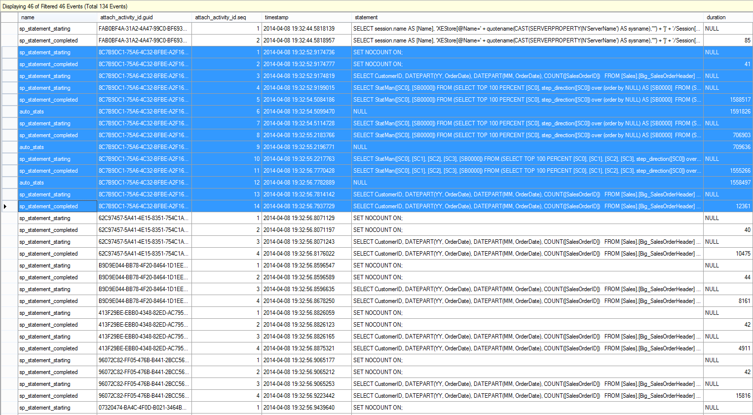
Example

Consider the simple task of counting the rows in a table, using the obvious single-statement query. Under locking read committed isolation with row-locking granularity, our query will take a shared lock on the first row, read it, release the shared lock, move on to the next row, and so on until it reaches the end of the structure it is reading. For the sake of this example, assume our query is reading an index b-tree in ascending key order (though it could just as well use a descending order, or any other strategy).

Since only a single row is share-locked at any given moment in time, it is clearly possible for concurrent transactions to modify the unlocked rows in the index our query is traversing. If these concurrent modifications change index key values, they will cause rows to move around within the index structure. With that possibility in mind, the diagram below illustrates two problematic scenarios that can occur:

The uppermost arrow shows a row we have already counted having its index key concurrently modified so that the row moves ahead of the current scan position in the index, meaning the row will be counted twice. The second arrow shows a row our scan has not encountered yet moving behind the scan position, meaning the row will not be counted at all.

Not a point-in-time view

The previous section showed how locking read committed can miss data completely, or count the same item multiple times (more than twice, if we are unlucky). The third bullet point in the list of unexpected behaviours stated that locking read committed does not provide a point-in-time view of the data either.

The reasoning behind that statement should now be easy to see. Our counting query, for example, could easily read data that was inserted by concurrent transactions after our query started executing. Equally, data that our query sees might be modified by concurrent activity after our query starts and before it completes. Finally, data we have read and counted might be deleted by a concurrent transaction before our query completes.

Clearly, the data seen by a statement or transaction running under locking read committed isolation corresponds to no single state of the database at any particular point in time. The data we encounter might well be from a variety of different points in time, with the only common factor being that each item represented the latest committed value of that data at the time it was read (though it might well have changed or disappeared since).

How serious are these problems?

This all might seem like a pretty woolly state of affairs if you are used to thinking of your single-statement queries and explicit transactions as logically executing instantaneously, or as running against a single committed point-in-time state of the database when using the default SQL Server isolation level. It certainly does not fit well with the concept of isolation in the ACID sense.

Given the apparent weakness of the guarantees provided by locking read committed isolation, you might start to wonder how any of your production T-SQL code has ever worked properly! Of course, we can accept that using an isolation level below serializable means we give up full ACID transaction isolation in return for other potential benefits, but just how serious can we expect these issues to be in practice?

Missing and double-counted rows

These first two issues essentially rely on concurrent activity changing keys in an index structure that we are currently scanning. Note that scanning here includes the partial range scan portion of an index seek, as well as the familiar unrestricted index or table scan.

If we are (range) scanning an index structure whose keys are not typically modified by any concurrent activity, these first two issues should not be much of a practical problem. It is difficult to be certain about this though, because query plans can change to use a different access method, and the new searched index might incorporate volatile keys.

We also have to bear in mind that many production queries only really need an approximate or best-effort answer to some types of question anyway. The fact that some rows are missing or double-counted might not matter much in the broader scheme of things. On a system with many concurrent changes, it might even be difficult to be sure that the result was inaccurate, given that the data changes so frequently. In that sort of situation, a roughly-correct answer might be good enough for the purposes of the data consumer.

No point-in-time view

The third issue (the question of a so-called 'consistent' point-in-time view of the data) also comes down to the same sort of considerations. For reporting purposes, where inconsistencies tend to result in awkward questions from the data consumers, a snapshot view is frequently preferable. In other cases, the sort of inconsistencies arising from the lack of a point-in-time view of the data may well be tolerable.

Problematic scenarios

There are also plenty of cases where the listed concerns will be important. For example, if you write code that enforces business rules in T-SQL, you need to be careful to select an isolation level (or take other suitable action) to guarantee correctness. Many business rules can be enforced using foreign keys or constraints, where the intricacies of isolation level selection are handled automatically for you by the database engine. As a general rule of thumb, using the built-in set of declarative integrity features is preferable to building your own rules in T-SQL.

There is another broad class of query that does not quite enforce a business rule per se, but which nevertheless might have unfortunate consequences when run at the default locking read committed isolation level. These scenarios are not always as obvious as the often-quoted examples of transferring money between bank accounts, or ensuring that the balance over a number of linked accounts never drops below zero. For example, consider the following query that identifies overdue invoices as an input to some process that sends out sternly-worded reminder letters:

INSERT dbo.OverdueInvoices
SELECT I.InvoiceNumber
FROM dbo.Invoices AS INV
WHERE INV.TotalDue >
(
    SELECT SUM(P.Amount)
    FROM dbo.Payments AS P
    WHERE P.InvoiceNumber = I.InvoiceNumber
);

Clearly we would not want to send a letter to someone who had fully paid their invoice in instalments, simply because concurrent database activity at the time our query ran meant we calculated an incorrect sum of payments received. Real queries on real production systems are frequently much more complex than the simple example above, of course.

To finish up for today, take a look at the following query and see if you can spot how many opportunities there are for something unintended to occur, if several such queries are run concurrently at the locking read committed isolation level (perhaps while other unrelated transactions are also modifying the Cases table):

-- Allocate the oldest unallocated case ID to 
-- the current case worker, while ensuring
-- the worker never has more than three
-- active cases at once.
UPDATE dbo.Cases
SET WorkerID = @WorkerID
WHERE 
    CaseID = 
    (
        -- Find the oldest unallocated case ID
        SELECT TOP (1)
            C2.CaseID
        FROM dbo.Cases AS C2
        WHERE 
            C2.WorkerID IS NULL
        ORDER BY 
            C2.DateCreated DESC
    )
    AND
    (
        SELECT COUNT_BIG(*) 
        FROM dbo.Cases AS C3
        WHERE C3.WorkerID = @WorkerID
    ) < 3;

Once you start looking for all the little ways a query can go wrong at this isolation level, it can be hard to stop. Bear in mind the caveats noted previously around the real need for completely isolated and point-in-time accurate results. It is perfectly fine to have queries that return good enough results, so long as you are aware of the trade-offs you are making by using read committed.

Next Time

The next part in this series looks at the second physical implementation of read committed isolation available in SQL Server, read committed snapshot isolation.

Delayed Durability is a late-breaking but interesting feature in SQL Server 2014; the high-level elevator pitch of the feature is, quite simply:

"Trade durability for performance."

Some background first. By default, SQL Server uses a write-ahead log (WAL), which means that changes are written to the log before they are allowed to be committed. In systems where transaction log writes become the bottleneck, and where there is a moderate tolerance for data loss, you now have the option to temporarily suspend the requirement to wait for the log flush and acknowledgement. This happens to quite literally take the D out of ACID, at least for a small portion of data (more on this later).

You kind of already make this sacrifice now. In full recovery mode, there is always some risk of data loss, it's just measured in terms of time rather than size. For example, if you back up the transaction log every five minutes, you could lose up to just under 5 minutes of data if something catastrophic happened. I'm not talking simple failover here, but let's say the server literally catches on fire or someone trips over the power cord – the database may very well be unrecoverable and you may have to go back to the point in time of the last log backup. And that's assuming you are even testing your backups by restoring them somewhere – in the event of a critical failure you may not have the recovery point you think you have. We tend not to think about this scenario, of course, because we never expect bad things™ to happen.

How it works

Delayed durability enables write transactions to continue running as if the log had been flushed to disk; in reality, the writes to disk have been grouped and deferred, to be handled in the background. The transaction is optimistic; it assumes that the log flush will happen. The system uses a 60KB chunk of log buffer, and attempts to flush the log to disk when this 60KB block is full. You can set this option at the database level, at the individual transaction level, or – in the case of natively compiled procedures in In-Memory OLTP – at the procedure level. The database setting wins in the case of a conflict; for example, if the database is set to disabled, trying to commit a transaction using the delayed option will simply be ignored, with no error message. Also, some transactions are always fully durable, regardless of database settings or commit settings; for example, system transactions, cross-database transactions, and operations involving FileTable, Change Tracking and Change Data Capture.

At the database level, you can use:

ALTER DATABASE dbname SET DELAYED_DURABILITY = DISABLED | ALLOWED | FORCED;

If you set it to ALLOWED, this means that any individual transaction can use Delayed Durability; FORCED means that all transactions that can use Delayed Durability will (the exceptions above are still relevant in this case). You will likely want to use ALLOWED rather than FORCED – but the latter can be useful in the case of an existing application where you want to use this option throughout and also minimize the amount of code that has to be touched. An important thing to note about ALLOWED is that fully durable transactions may have to wait longer, as they will force the flush of any delayed durable transactions first.

At the transaction level, you can say:

COMMIT TRANSACTION WITH (DELAYED_DURABILITY = ON);

And in an In-Memory OLTP natively-compiled procedure, you can add the following option to the BEGIN ATOMIC block:

BEGIN ATOMIC WITH (DELAYED_DURABILITY = ON, ...)

A common question is around what happens with locking and isolation semantics. Nothing changes, really. Locking and blocking still happen, and transactions are committed in the same way and with the same rules. The only difference is that, by allowing the commit to occur without waiting for the log to flush to disk, any related locks are released that much sooner.

When You Should Use It

In addition to the benefit you get from allowing the transactions to proceed without waiting for the log write to happen, you also get fewer log writes of larger sizes. This can work out very well if your system has a high proportion of transactions that are actually smaller than 60KB, and particularly when the log disk is slow (though I found similar benefits on SSD and traditional HDD). It doesn't work out so well if your transactions are, for the most part, larger than 60KB, if they are typically long-running, or if you have high throughput and high concurrency. What can happen here is that you can fill the entire log buffer before the flush finishes, which just means transferring your waits to a different resource and, ultimately, not improving the perceived performance by the users of the application.

In other words, if your transaction log is not currently a bottleneck, don't turn this feature on. How can you tell if your transaction log is currently a bottleneck? The first indicator would be high WRITELOG waits, particularly when coupled with PAGEIOLATCH_**. Paul Randal (@PaulRandal) has a great four-part series on identifying transaction log problems, as well as configuring for optimal performance:

• Trimming the Transaction Log Fat
• Trimming More Transaction Log Fat
• Transaction Log Configuration Issues
• Transaction Log Monitoring

Also see this blog post from Kimberly Tripp (@KimberlyLTripp), 8 Steps to Better Transaction Log Throughput, and the SQL CAT team's blog post, Diagnosing Transaction Log Performance Issues and Limits of the Log Manager.

This investigation may lead you to the conclusion that Delayed Durability is worth looking into; it may not. Testing your workload will be the most reliable way to know for sure. Like many other additions in recent versions of SQL Server (*cough* Hekaton), this feature is NOT designed to improve every single workload – and as noted above, it can actually make some workloads worse. See this blog post by Simon Harvey for some other questions you should ask yourself about your workload to determine if it is feasible to sacrifice some durability to achieve better performance.

Potential for data loss

I'm going to mention this several times, and add emphasis every time I do: You need to be tolerant to data loss. Under a well-performing disk, the maximum you should expect to lose in a catastrophe – or even a planned and graceful shutdown – is up to one full block (60KB). However, in the case where your I/O subsystem can't keep up, it is possible that you could lose as much as the entire log buffer (~7MB).

To clarify, from the documentation (emphasis mine):

So it is very important that you weigh your data loss risk with your need to alleviate transaction log performance issues. If you run a bank or anything dealing with money, it may be much safer and more appropriate for you to move your log to faster disk than to roll the dice using this feature. If you are trying to improve the response time in your Web Gamerz Chat Room application, maybe the risk is less severe.

You can control this behavior to some degree in order to minimize your risk of data loss. You can force all delayed durable transactions to be flushed to disk in one of two ways:

1. Commit any fully durable transaction.
2. Call sys.sp_flush_log manually.

This allows you to revert to controlling data loss in terms of time, rather than size; you could schedule the flush every 5 seconds, for example. But you will want to find your sweet spot here; flushing too often can offset the Delayed Durability benefit in the first place. In any case, you will still need to be tolerant to data loss, even if it is only <n> seconds' worth.

You would think that CHECKPOINT might help here, but this operation actually does not technically guarantee the log will be flushed to disk.

Interaction with HA/DR

You might wonder how Delayed Durablity functions with HA/DR features such as log shipping, replication, and Availability Groups. With most of these it works unchanged. Log shipping and replication will replay the log records that have been hardened, so the same potential for data loss exists there. With AGs in asynchronous mode, we're not waiting for the secondary acknowledge anyway, so it will behave the same as today. With synchronous, however, we can't commit on the primary until the transaction is committed and hardened to the remote log. Even in that scenario we may have some benefit locally by not having to wait for the local log to write, we still have to wait for the remote activity. So in that scenario there is less benefit, and potentially none; except perhaps in the rare scenario where the primary's log disk is really slow and the secondary's log disk is really fast. I suspect the same conditions hold true for sync/async mirroring, but you won't get any official commitment from me about how a shiny new feature works with a deprecated one. :-)

Performance Observations

This wouldn't be much of a post here if I didn't show some actual performance observations. I set up 8 databases to test the effects of two different workload patterns with the following attributes:

• Recovery model: simple vs. full
• Log location: SSD vs. HDD
• Durability: delayed vs. fully durable

I am really, really, really lazyefficient about this kind of thing. Since I want to avoid repeating the same operations within each database, I created the following table temporarily in model:

USE model;
GO
 
CREATE TABLE dbo.TheTable
(
  TheID INT IDENTITY(1,1) PRIMARY KEY,
  TheDate DATETIME NOT NULL DEFAULT CURRENT_TIMESTAMP,
  RowGuid UNIQUEIDENTIFIER NOT NULL DEFAULT NEWID()
);

Then I built a set of dynamic SQL command to builds these 8 databases, rather than create the databases individually and then muck with the settings:

-- C and D are SSD, G is HDD
 
DECLARE @sql NVARCHAR(MAX) = N'';
 
;WITH l AS (SELECT l FROM (VALUES('D'),('G')) AS l(l)),
r AS (SELECT r FROM (VALUES('FULL'),('SIMPLE')) AS r(r)),
d AS (SELECT d FROM (VALUES('FORCED'),('DISABLED')) AS d(d)),
x AS (SELECT l.l, r.r, d.d, n = CONVERT(CHAR(1),ROW_NUMBER() OVER 
  (ORDER BY d.d DESC, l.l)) FROM l CROSS JOIN r CROSS JOIN d)
SELECT @sql += N'
CREATE DATABASE dd' + n + ' ON '
+ '(name = ''dd' + n + '_data'','
+ ' filename = ''C:\SQLData\dd' + n + '.mdf'', size = 1024MB)
LOG ON (name = ''dd' + n + '_log'','
+ ' filename = ''' + l + ':\SQLLog\dd' + n + '.ldf'', size = 1024MB);
  ALTER DATABASE dd' + n + ' SET RECOVERY ' + r  + ';
  ALTER DATABASE dd' + n + ' SET DELAYED_DURABILITY = ' + d + ';'
FROM x ORDER BY d, l;
 
PRINT @sql;
-- EXEC sp_executesql @sql;

Feel free to run this code yourself (with the EXEC still commented out) to see that this would create 4 databases with Delayed Durability OFF (two in FULL recovery, two in SIMPLE, one of each with log on slow disk, and one of each with log on SSD). Repeat that pattern for 4 databases with Delayed Durability FORCED – I did this to simplify the code in the test, rather than to reflect what I would do in real life (where I would likely want to treat some transactions as critical, and some as, well, less than critical).

For sanity checking, I ran the following query to ensure that the databases had the right matrix of attributes:

SELECT d.name, d.recovery_model_desc, d.delayed_durability_desc, 
  log_disk = CASE WHEN mf.physical_name LIKE N'D%' THEN 'SSD' else 'HDD' END
FROM sys.databases AS d
INNER JOIN sys.master_files AS mf
ON d.database_id = mf.database_id
WHERE d.name LIKE N'dd[1-8]'
AND mf.[type] = 1; -- log

Results:

Relevant configuration of the 8 test databases

I also ran the test cleanly multiple times to ensure that a 1 GB data file and 1 GB log file would be sufficient to run the entire set of workloads without introducing any autogrowth events into the equation. As a best practice, I routinely go out of my way to ensure customers' systems have enough allocated space (and proper alerts built in) such that no growth event ever occurs at an unexpected time. In the real world I know this doesn't always happen, but it is ideal.

I set up the system to be monitored with SQL Sentry Performance Advisor – this would allow me to easily show most of the performance metrics I wanted to highlight. But I also created a temporary table to store batch metrics including duration and very specific output from sys.dm_io_virtual_file_stats:

SELECT test = 1, cycle = 1, start_time = GETDATE(), * 
INTO #Metrics 
FROM sys.dm_io_virtual_file_stats(DB_ID('dd1'), 2) WHERE 1 = 0;

This would allow me to record the start and finish time of each individual batch, and measure deltas in the DMV between start time and end time (only reliable in this case because I know I'm the only user on the system).

Lots of small transactions

The first test I wanted to perform was a lot of small transactions. For each database, I wanted to end up with 500,000 separate batches of a single insert each:

INSERT #Metrics SELECT 1, 1, GETDATE(), * 
  FROM sys.dm_io_virtual_file_stats(DB_ID('dd1'), 2);
GO
INSERT dbo.TheTable DEFAULT VALUES;
GO 500000
INSERT #Metrics SELECT 1, 2, GETDATE(), * 
  FROM sys.dm_io_virtual_file_stats(DB_ID('dd1'), 2);

Remember, I try to be lazyefficient about this kind of thing. So to generate the code for all 8 databases, I ran this:

;WITH x AS 
(
  SELECT TOP (8) number FROM master..spt_values 
  WHERE type = N'P' ORDER BY number
)
SELECT CONVERT(NVARCHAR(MAX), N'') + N'
INSERT #Metrics SELECT 1, 1, GETDATE(), * 
  FROM sys.dm_io_virtual_file_stats(DB_ID(''dd' + RTRIM(number+1) + '''), 2);
GO
INSERT dbo.TheTable DEFAULT VALUES;
GO 500000
INSERT #Metrics SELECT 1, 2, GETDATE(), * 
  FROM sys.dm_io_virtual_file_stats(DB_ID(''dd' + RTRIM(number+1) + '''), 2);'
FROM x;

I ran this test and then looked at the #Metrics table with the following query:

SELECT 
  [database] = db_name(m1.database_id),
  num_writes = m2.num_of_writes - m1.num_of_writes, 
  write_bytes = m2.num_of_bytes_written - m1.num_of_bytes_written,
  bytes_per_write = (m2.num_of_bytes_written - m1.num_of_bytes_written)*1.0
    /(m2.num_of_writes - m1.num_of_writes),
  io_stall_ms = m2.io_stall_write_ms - m1.io_stall_write_ms,
  m1.start_time,
  end_time = m2.start_time,
  duration = DATEDIFF(SECOND, m1.start_time, m2.start_time)
FROM #Metrics AS m1
INNER JOIN #Metrics AS m2
ON m1.database_id = m2.database_id
WHERE m1.cycle = 1 AND m2.cycle = 2
AND m1.test = 1 AND m2.test = 1;

This yielded the following results (and I confirmed through multiple tests that the results were consistent):

database	writes	bytes	bytes/write	io_stall_ms	start_time	end_time	duration (seconds)
dd1	8,068	261,894,656	32,460.91	6,232	2014-04-26 17:20:00	2014-04-26 17:21:08	68
dd2	8,072	261,682,688	32,418.56	2,740	2014-04-26 17:21:08	2014-04-26 17:22:16	68
dd3	8,246	262,254,592	31,803.85	3,996	2014-04-26 17:22:16	2014-04-26 17:23:24	68
dd4	8,055	261,688,320	32,487.68	4,231	2014-04-26 17:23:24	2014-04-26 17:24:32	68
dd5	500,012	526,448,640	1,052.87	35,593	2014-04-26 17:24:32	2014-04-26 17:26:32	120
dd6	500,014	525,870,080	1,051.71	35,435	2014-04-26 17:26:32	2014-04-26 17:28:31	119
dd7	500,015	526,120,448	1,052.20	50,857	2014-04-26 17:28:31	2014-04-26 17:30:45	134
dd8	500,017	525,886,976	1,051.73	49,680	2014-04-26 17:30:45	2014-04-26 17:32:58	133

Small transactions: Duration and results from sys.dm_io_virtual_file_stats

Definitely some interesting observations here:

• Number of individual write operations was very small for the Delayed Durability databases (~60X for traditional).
• Total number of bytes written was cut in half using Delayed Durability (I presume because all of the writes in the traditional case contained a lot of wasted space).
• The number of bytes per write was a lot higher for Delayed Durability. This was not overly surprising, since the whole purpose of the feature is to bundle writes together in larger batches.
• The total duration of I/O stalls was volatile, but roughly an order of magnitude lower for Delayed Durability. The stalls under fully durable transactions were much more sensitive to the type of disk.
• If anything hasn't convinced you so far, the duration column is very telling. Fully durable batches that take two minutes are more are cut almost in half.

The start/end time columns allowed me to focus on the Performance Advisor dashboard for the precise period where these transactions were happening, where we can draw a lot of additional visual indicators:


SQL Sentry Performance Advisor dashboard – click to enlarge

Further observations here:

• On several graphs, you can clearly see exactly when the non-Delayed Durability portion of the batch took over (~5:24:32 PM).
• There is no observable impact to CPU or memory when using Delayed Durability.
• You can see a tremendous impact to batches/transactions per second in the first graph under SQL Server Activity.
• SQL Server waits go through the roof when the fully durable transactions started. These were comprised almost exclusively of WRITELOG waits, with a small number of PAGEIOLOATCH_EX and PAGEIOLATCH_UP waits for good measure.
• The total number of log flushes throughout the Delayed Durability operations was quite small (low 100s/sec), while this jumped to over 4,000/sec for the traditional behavior (and slightly lower for the HDD duration of the test).

Fewer, larger transactions

For the next test, I wanted to see what would happen if we performed fewer operations, but made sure each statement affected a larger amount of data. I wanted this batch to run against each database:

CREATE TABLE dbo.Rnd
(
  batch TINYINT,
  TheID INT
);
 
INSERT dbo.Rnd SELECT TOP (1000) 1, TheID FROM dbo.TheTable ORDER BY NEWID();
INSERT dbo.Rnd SELECT TOP (10)   2, TheID FROM dbo.TheTable ORDER BY NEWID();
INSERT dbo.Rnd SELECT TOP (300)  3, TheID FROM dbo.TheTable ORDER BY NEWID();
GO
 
INSERT #Metrics SELECT 1, GETDATE(), * 
  FROM sys.dm_io_virtual_file_stats(DB_ID('dd1'), 2);
GO
UPDATE t SET TheDate = DATEADD(MINUTE, 1, TheDate)
  FROM dbo.TheTable AS t
  INNER JOIN dbo.Rnd AS r
  ON t.TheID = r.TheID
  WHERE r.batch = 1;
GO 10000
UPDATE t SET RowGuid = NEWID()
  FROM dbo.TheTable AS t
  INNER JOIN dbo.Rnd AS r
  ON t.TheID = r.TheID
  WHERE r.batch = 2;
GO 10000
DELETE dbo.TheTable WHERE TheID IN (SELECT TheID   FROM dbo.Rnd WHERE batch = 3);
DELETE dbo.TheTable WHERE TheID IN (SELECT TheID+1 FROM dbo.Rnd WHERE batch = 3);
DELETE dbo.TheTable WHERE TheID IN (SELECT TheID-1 FROM dbo.Rnd WHERE batch = 3);
GO
INSERT #Metrics SELECT 2, GETDATE(), * 
  FROM sys.dm_io_virtual_file_stats(DB_ID('dd1'), 2);

So again I used the lazy method to produce 8 copies of this script, one per database:

;WITH x AS (SELECT TOP (8) number FROM master..spt_values WHERE type = N'P' ORDER BY number)
SELECT N'
USE dd' + RTRIM(Number+1) + ';
GO
 
CREATE TABLE dbo.Rnd
(
  batch TINYINT,
  TheID INT
);
 
INSERT dbo.Rnd SELECT TOP (1000) 1, TheID FROM dbo.TheTable ORDER BY NEWID();
INSERT dbo.Rnd SELECT TOP (10)   2, TheID FROM dbo.TheTable ORDER BY NEWID();
INSERT dbo.Rnd SELECT TOP (300)  3, TheID FROM dbo.TheTable ORDER BY NEWID();
GO
 
INSERT #Metrics SELECT 2, 1, GETDATE(), * 
  FROM sys.dm_io_virtual_file_stats(DB_ID(''dd' + RTRIM(number+1) + ''', 2);
GO
UPDATE t SET TheDate = DATEADD(MINUTE, 1, TheDate)
  FROM dbo.TheTable AS t
  INNER JOIN dbo.rnd AS r
  ON t.TheID = r.TheID
  WHERE r.cycle = 1;
GO 10000
UPDATE t SET RowGuid = NEWID()
  FROM dbo.TheTable AS t
  INNER JOIN dbo.rnd AS r
  ON t.TheID = r.TheID
  WHERE r.cycle = 2;
GO 10000
DELETE dbo.TheTable WHERE TheID IN (SELECT TheID   FROM dbo.rnd WHERE cycle = 3);
DELETE dbo.TheTable WHERE TheID IN (SELECT TheID+1 FROM dbo.rnd WHERE cycle = 3);
DELETE dbo.TheTable WHERE TheID IN (SELECT TheID-1 FROM dbo.rnd WHERE cycle = 3);
GO
INSERT #Metrics SELECT 2, 2, GETDATE(), * 
  FROM sys.dm_io_virtual_file_stats(DB_ID(''dd' + RTRIM(number+1) + '''), 2);'
FROM x;

I ran this batch, then changed the query against #Metrics above to look at the second test instead of the first. The results:

database	writes	bytes	bytes/write	io_stall_ms	start_time	end_time	duration (seconds)
dd1	20,970	1,271,911,936	60,653.88	12,577	2014-04-26 17:41:21	2014-04-26 17:43:46	145
dd2	20,997	1,272,145,408	60,587.00	14,698	2014-04-26 17:43:46	2014-04-26 17:46:11	145
dd3	20,973	1,272,982,016	60,696.22	12,085	2014-04-26 17:46:11	2014-04-26 17:48:33	142
dd4	20,958	1,272,064,512	60,695.89	11,795	2014-04-26 17:48:33	2014-04-26 17:50:56	143
dd5	30,138	1,282,231,808	42,545.35	7,402	2014-04-26 17:50:56	2014-04-26 17:53:23	147
dd6	30,138	1,282,260,992	42,546.31	7,806	2014-04-26 17:53:23	2014-04-26 17:55:53	150
dd7	30,129	1,281,575,424	42,536.27	9,888	2014-04-26 17:55:53	2014-04-26 17:58:25	152
dd8	30,130	1,281,449,472	42,530.68	11,452	2014-04-26 17:58:25	2014-04-26 18:00:55	150

Larger transactions: Duration and results from sys.dm_io_virtual_file_stats

This time, the impact of Delayed Durability is much less noticeable. We see a slightly smaller number of write operations, at a slightly larger number of bytes per write, with the total bytes written almost identical. In this case we actually see the I/O stalls are higher for Delayed Durability, and this likely accounts for the fact that the durations were almost identical as well.

From the Performance Advisor dashboard, we some similarities with the previous test, and some stark differences as well:


SQL Sentry Performance Advisor dashboard – click to enlarge

One of the big differences to point out here is that the delta in wait stats is not quite as pronounced as with the previous test – there is still a much higher frequency of WRITELOG waits for the fully durable batches, but nowhere near the levels seen with the smaller transactions. Another thing you can spot immediately is that the previously observed impact on batches and transactions per second is no longer present. And finally, while there are more log flushes with fully durable transactions than when delayed, this disparity is far less pronounced than with the smaller transactions.

Conclusion

It should be clear that there are certain workload types that may benefit greatly from Delayed Durability – provided, of course, that you have a tolerance for data loss. This feature is not restricted to In-Memory OLTP, is available on all editions of SQL Server 2014, and can be implemented with little to no code changes. It can certainly be a powerful technique if your workload can support it. But again, you will need to test your workload to be sure that it will benefit from this feature, and also strongly consider whether this increases your exposure to the risk of data loss.

As an aside, this may seem to the SQL Server crowd like a fresh new idea, but in truth Oracle introduced this as "Asynchronous Commit" in 2006 (see COMMIT WRITE ... NOWAIT as documented here and blogged about in 2007). And the idea itself has been around for nearly 3 decades; see Hal Berenson's brief chronicle of its history.

Next Time

One idea that I have batted around is to try to improve the performance of tempdb by forcing Delayed Durability there. One special property of tempdb that makes it such a tempting candidate is that it is transient by nature – anything in tempdb is designed, explicitly, to be tossable in the wake of a wide variety of system events. I am saying this now without having any idea if there is a workload shape where this will work out well; but I do plan to try it out, and if I find anything interesting, you can be sure I will post about it here.

In my previous post, I explored different methods to track automatic updates to statistics to determine if they were affecting query performance. In the latter half of the post I included options, one of which was to enable the Auto Update Statistics Asynchronously database setting. In this post, I want to look at how query performance changes when the automatic update does occur prior to query execution, and what happens to performance if the update is asynchronous.

The Set Up

I started with a copy of the AdventureWorks2012 database, and then created a copy of the SalesOrderHeader table with over 200 million rows using this script. The table has a clustered index on SalesOrderID, and a nonclustered index on CustomerID, OrderDate, SubTotal. [Note: if you are going to do repeated tests, take a backup of this database at this point to save yourself some time]. After loading the data and creating the nonclustered index, I verified row count and calculated how many rows (approximately) would need to be modified to invoke an automatic update.

SELECT
OBJECT_NAME([p].[object_id]) [TableName],
[si].[name] [IndexName],
[au].[type_desc] [Type],
[p].[rows] [RowCount],
([p].[rows]*.20) + 500 [UpdateThreshold],
[au].total_pages [PageCount],
(([au].[total_pages]*8)/1024)/1024 [TotalGB]
FROM [sys].[partitions] [p]
JOIN [sys].[allocation_units] [au] ON [p].[partition_id] = [au].[container_id]
JOIN [sys].[indexes] [si] on [p].[object_id] = [si].object_id and [p].[index_id] = [si].[index_id]
WHERE [p].[object_id] = OBJECT_ID(N'Sales.Big_SalesOrderHeader');

Big_SalesOrderHeader CIX and NCI Information

I also verified the current statistics header for the index:

DBCC SHOW_STATISTICS ('Sales.Big_SalesOrderHeader',[IX_Big_SalesOrderHeader_CustomerID_OrderDate_SubTotal]);

NCI Statistics: At Start

I then created the stored procedure that I would use for testing. It’s a straightforward procedure that queries Sales.Big_SalesOrderHeader, and aggregates sales data by CustomerID and OrderDate for analysis:

CREATE PROCEDURE Sales.usp_GetCustomerStats
@CustomerID INT,
@StartDate DATETIME,
@EndDate DATETIME
AS
BEGIN
  SET NOCOUNT ON;
 
  SELECT CustomerID, DATEPART(YEAR, OrderDate), DATEPART(MONTH, OrderDate), COUNT([SalesOrderID]) as Computed
    FROM [Sales].[Big_SalesOrderHeader]
    WHERE CustomerID = @CustomerID
    AND OrderDate BETWEEN @StartDate and @EndDate
    GROUP BY CustomerID, DATEPART(YEAR, OrderDate), DATEPART(MONTH, OrderDate)
    ORDER BY DATEPART(YEAR, OrderDate), DATEPART(MONTH, OrderDate);
END

Finally, before executing the stored procedure, I created an Extended Events session so I could track query duration using sp_statement_starting and sp_statement_completed. I also added the auto_stats event, because even though I did not expect an update to occur, I wanted to use this same session definition later.

CREATE EVENT SESSION [StatsUpdate_QueryPerf]
ON SERVER
ADD EVENT sqlserver.auto_stats,
ADD EVENT sqlserver.sp_statement_completed(
SET collect_statement=(1)
),
ADD EVENT sqlserver.sp_statement_starting
ADD TARGET package0.event_file(
SET filename=N'C:\temp\StatsUpdate_QueryPerf.xel'
)
WITH (MAX_MEMORY=4096 KB,EVENT_RETENTION_MODE=ALLOW_SINGLE_EVENT_LOSS,MAX_DISPATCH_LATENCY=30 SECONDS,
MAX_EVENT_SIZE=0 KB,MEMORY_PARTITION_MODE=NONE,TRACK_CAUSALITY=ON,STARTUP_STATE=OFF);
GO

The Test

I started the Extended Events session, and then executed the stored procedure multiple times, using different CustomerIDs:

ALTER EVENT SESSION [StatsUpdate_QueryPerf]
ON SERVER
STATE = START;
GO
 
EXEC Sales.usp_GetCustomerStats 11331, '2012-08-01 00:00:00.000', '2012-08-31 23:59:59.997'
GO
EXEC Sales.usp_GetCustomerStats 11330, '2013-01-01 00:00:00.000', '2013-01-31 23:59:59.997'
GO
EXEC Sales.usp_GetCustomerStats 11506, '2012-11-01 00:00:00.000', '2012-11-30 23:59:59.997'
GO
EXEC Sales.usp_GetCustomerStats 17061, '2013-01-01 00:00:00.000', '2013-01-31 23:59:59.997'
GO
EXEC Sales.usp_GetCustomerStats 11711, '2013-03-01 00:00:00.000', '2013-03-31 23:59:59.997'
GO
EXEC Sales.usp_GetCustomerStats 15131, '2013-02-01 00:00:00.000', '2013-02-28 23:59:59.997'
GO
EXEC Sales.usp_GetCustomerStats 29837, '2012-10-01 00:00:00.000', '2012-10-31 23:59:59.997'
GO
EXEC Sales.usp_GetCustomerStats 15750, '2013-03-01 00:00:00.000', '2013-03-31 23:59:59.997'
GO

I verified the execution count, and the plan, by querying the procedure cache:

SELECT
OBJECT_NAME([st].[objectid]),
[st].[text],
[qs].[execution_count],
[qs].[creation_time],
[qs].[last_execution_time],
[qs].[min_worker_time],
[qs].[max_worker_time],
[qs].[min_logical_reads],
[qs].[max_logical_reads],
[qs].[min_elapsed_time],
[qs].[max_elapsed_time],
[qp].[query_plan]
FROM [sys].[dm_exec_query_stats] [qs]
CROSS APPLY [sys].[dm_exec_sql_text]([qs].plan_handle) [st]
CROSS APPLY [sys].[dm_exec_query_plan]([qs].plan_handle) [qp]
WHERE [st].[text] LIKE '%usp_GetCustomerStats%'
AND OBJECT_NAME([st].[objectid]) IS NOT NULL;

Plan Cache: At Start

Query Plan for Stored Procedure, using SQL Sentry Plan Explorer

I could see that the plan was created at 2014-04-08 18:59:39.850. With the plan in cache, I stopped the Extended Events session:

ALTER EVENT SESSION [StatsUpdate_QueryPerf]
ON SERVER
STATE = STOP;

Next I added about 47 million rows of data to the table using this script, well over the threshold necessary to invalidate the current statistics. After adding the data, I verified the number of rows in the table:

Big_SalesOrderHeader CI: After Data Load

Before I re-ran my stored procedure, I checked the plan cache to make sure nothing had changed, and verified that statistics had not yet updated. Remember, even though the statistics were invalidated at this point, they will not update until a query that uses the statistic is executed (for reference: Understanding When Statistics Will Automatically Update). For the final step, I started the Extended Events session again, and then ran the stored procedure multiple times.  After those executions, I checked the plan cache again:

Plan Cache: After Data Load

The execution_count is 8 again, and if we look at the create_time of the plan, we can see it’s changed to 2014-04-08 19:32:52.913. If we check the plan, we can see that it is the same, even though the plan was recompiled:

Query Plan for Stored Procedure, using SQL Sentry Plan Explorer

Analysis of Extended Events Output

I took the first Extended Events file – before data was loaded – and opened it in SSMS, then applied a filter so that only statements from the stored procedure were listed:

Extended Events Output: After Initial SP Execution

You can see that there are eight (8) executions of the stored procedure, with query durations that vary slightly.

I took the second Extended Events file – after data was loaded – opened it SSMS, and filtered again so that only statements from the stored procedure, as well as auto_stats events, were listed:

Extended Events Output: SP Execution After Data Load

The output is truncated, as it is not all needed to show the main result. The blue highlighted entries represent the first execution of the stored procedure, and note that there are multiple steps – the update to statistics is part of the execution. The SELECT statement starts (attach_activity_id.seq = 3), and the updates to statistics then execute. In our example, we actually have updates to three statistics. Once the last update completes (attach_activity_id.seq = 11), then the stored procedure starts and completes (attach_activity_id.seq = 13 and attach_activity_id.seq = 14). Interestingly enough, there is a second sp_statement_starting event for the stored procedure (presumably the first one is disregarded), so the total duration for the stored procedure is calculated without the update to statistics.

In this scenario, having statistics automatically update immediately – that is, when a query that uses invalidated statistics executes – causes the query to run longer, even though query duration based on the sp_statement_completed event is still less than 14000. The end result is that there is no benefit to query performance, as the plan is exactly same before and after the statistics update. In this scenario, the query plan and execution duration do not change after more data is added to the table, so the update to statistics only hinders its performance. Now let’s see what happens when we enable the Auto Update Statistics Asynchronously option.

The Test, Version 2

We start by restoring to the backup that I took before we started the first test. I recreated the stored procedure and then changed the database option to update statistics asynchronously:

USE [master];
GO
ALTER DATABASE [AdventureWorks2012_Big] SET AUTO_UPDATE_STATISTICS_ASYNC ON WITH NO_WAIT
GO

I started the Extended Events session, and again executed the stored procedure multiple times, using different CustomerIDs:

ALTER EVENT SESSION [StatsUpdate_QueryPerf]
ON SERVER
STATE = START;
GO
 
EXEC Sales.usp_GetCustomerStats11331, '2012-08-01 00:00:00.000', '2012-08-31 23:59:59.997'
GO
EXEC Sales.usp_GetCustomerStats11330, '2013-01-01 00:00:00.000', '2013-01-31 23:59:59.997'
GO
EXEC Sales.usp_GetCustomerStats11506, '2012-11-01 00:00:00.000', '2012-11-30 23:59:59.997'
GO
EXEC Sales.usp_GetCustomerStats17061, '2013-01-01 00:00:00.000', '2013-01-31 23:59:59.997'
GO
EXEC Sales.usp_GetCustomerStats11711, '2013-03-01 00:00:00.000', '2013-03-31 23:59:59.997'
GO
EXEC Sales.usp_GetCustomerStats15131, '2013-02-01 00:00:00.000', '2013-02-28 23:59:59.997'
GO
EXEC Sales.usp_GetCustomerStats29837, '2012-10-01 00:00:00.000', '2012-10-31 23:59:59.997'
GO
EXEC Sales.usp_GetCustomerStats15750, '2013-03-01 00:00:00.000', '2013-03-31 23:59:59.997'
GO

I verified the execution count, and the plan, by querying the procedure cache:

Plan Cache: At Start, Test 2

Query Plan for Stored Procedure, using SQL Sentry Plan Explorer

For this test, the plan was created at 2014-04-08 21:15:55.490. I stopped the Extended Events session and again added about 47 million rows of data to the table, using the same query as before.

Once the data had been added, I checked the plan cache to make sure nothing had changed, and verified that statistics had not yet updated. Finally, I started the Extended Events session again, and then ran the stored procedure eight more times. A final peek into the plan cache showed execution_count at 16 and a create_time of 2014-04-08 21:15:55.490. The execution_count and create_time demonstrate that statistics have not updated, as the plan hasn't been flushed from cache yet (if it had, we would have a later create_time and an execution_count of 8).

Plan Cache: After Data Load, Test 2

If we open the Extended Events output from after the data load in SSMS, and again filter so we only see statements from the stored procedure, as well as auto_stats events, we find this (note that the output is broken into two screen shots):

Extended Events Output: Test 2, SP Execution After Data Load, part I

Extended Events Output: Test 2, SP Execution After Data Load, part II

The events for the execution of the first call of the stored procedure are highlighted in blue – they start at 2014-04-08 21:54:14.9480607 and there are seven (7) events. Note that there are three (3) auto_stats events, but none of them actually complete, as we saw when the Auto Update Statistics Asynchronously option was disabled. You'll notice that the automatic update does start for one of the statistics almost immediately (2014-04-08 21:54:14.9481288), and it's three events have the red text 'Stat Update #1' next to them. That statistics update finishes at 2014-04-08 21:54:16.5392219, just under two seconds after it starts, but after all other executions of the procedure have completed. This is why the execution_count from sys.dm_exec_query_stats shows 16. From the XE output, we can see that the other statistics updates then complete (Stat Update #2 and Stat Update #3). All of the updates are asynchronous to the initial stored procedure's execution.

Summary

As you can see, automatic updates to statistics have the potential to negatively affect query performance. The degree of impact will depend on the amount of data that has to be read to update the statistic, and the system resources. In some cases, query performance only increases by milliseconds and is most likely imperceptible to users. Other times, the duration can increase dramatically, which then affects end-user experience. In the case where the query plan does not change after an update to statistics, it is well worth considering enabling the Auto Update Statistics Asynchronously option, to mitigate the impact on query performance.

Just a few days before my session about Power Query at TechEd 2014, Microsoft released a new update that enables the scheduled data refresh of a Power Pivot workbook containing Power Query transformations.

This is a very good news, because it enables the data refresh of a number of different data sources. Even if the number of providers supported by this release is limited (only SQL Server and Oracle), you can use a SQL Server database as a bridge to access different data sources through views using Linked Server connections.

If you want to use this feature, first of all read carefully the Scheduled Data Refresh for Power Query blog post on MSDN web site. It guides you through are the steps required in order to enable the data source connection through the Data Management Gateway. As you will see, in reality you need to create the data source connections corresponding to the Power Query databases you use. Thus, in reality you might skip the data source configuration if you already have the corresponding databases enabled in the Power BI admin center. However, I suggest you to go through the steps described in that blog post at the beginning, because if the same database has two different drivers, it needs two different data sources. For this reason, I have a number of notes that might be helpful to avoid certain issues.

• Power Query uses the .NET Framework Data Provider for SQL Server and Oracle Data Provider for .NET, whereas Power Pivot by default creates a SQL Server connection using the SQL Server Native Client 11.0 (SQLNCLI11).
• Even if you already created a data source for a SQL Server database you refresh in a Power Pivot workbook, you have to create another data source for the same SQL Server database for Power Query, because you use two different drivers.
• You might consolidate these data sources to only one, by changing the data provide in the advanced options of a Power Pivot configuration, but I am not sure this is a good idea. I would keep the two version of data sources, one for each provider, in case I use the same database in both connections
• Power Query creates one connection string in Excel for each query you create. The connection string contains the entire transformation and when you copy it in the New Data Source page in Power BI admin, the internal query is analyzed to extract the required connection to SQL Server. If these connections are already configured as Power BI data sources, then you don’t need to do anything else. I suggest you to iterate all the queries you have following this step until you are confident of the internals and you are sure the required data sources are already available.
• Even if you create a single query in M language accessing to different databases, the referenced connections will be found and each database will have a separate data source configuration in Power BI. I was worried that loading multiple tables from different database on the same server would have produced a single data source enabling to access all the databases on the server, but luckily this does not happen and security is preserved!
• I spot an issue using certain DateTimeZone functions (DateTimeZone.FixedLocalNow, DateTimeZone.FixedUtcNow, DateTimeZone.LocalNow, and DateTimeZone.UtcNow) that seem not working with scheduled data refresh. You can read more about such issue in this thread on Power Query MSDN forum. I found a workaround using the Table.Buffer function, so that by stopping query folding the expression is not translated in SQL but evaluated directly by the Power Query engine. However, I hope this will be fixed soon.
• A Power Query transformation that contains only a script, without accessing to any data source, currently is not refreshed. This would be useful for generating a Date table, I opened this other thread about this issue on the forum, I hope there will be news on that, too.
• In the same thread you will find another tip: the literal in the form #literal, such as #table, are being mis-analyzed by scheduled refresh, but at least for this issue there are workarounds available, until the issue is not fixed by Microsoft.
• You can use SQL Server views based on linked servers to overcome the limitation of providers currently supported by Data Management Gateway (which is the component used by scheduled data refresh).
• Now that it is possible to publish SSIS packages as OData Feed Sources, you can expose a SQL Server view to Power BI, and accessing it from Power Pivot or Power Query, you can execute SSIS packages at refresh time. If the package is not too long to execute (it would timeout the connection), this is a smart way to arrange execution of some small “corporate ETL” in sync with the data refresh on Power BI, without relying on synchronized scheduling dates (which is always one more thing to maintain). This further extends the range of providers you can use with scheduled data refresh.

I would like to get more detailed errors when something goes wrong and scheduled data refresh stops, but this is a good start.

I was recently chatting with the current President of PASS, Thomas LaRock (Twitter | Blog), and Pieter Vanhove (Twitter | Blog), a prominent SQL Server consultant and expert in Belgium, about how I go about building and presenting a full-day technical seminar. In the SQL Server world, we tend to call these “pre-cons”, as in pre-conference seminar, because they’re typically offered as paid add-ons occurring prior to a full technical conference. We call them that even when they come at the end of the conference and, heck, when there’s no conference at all.

Kevin and Kendal Van Dyke preparing to kick off a session at the PASS Summit 2013

Personally, I have developed and delivered six different pre-cons over the years. Four are purely technical and two are professional development oriented. I keep them up to date and deliver around six per year these days, though I’ve done as many as ten in a single year. (But that was because I had a daughter’s wedding to pay for. Shameless plug – HIRE ME to deliver one of these in house.)

The Foundation of a Good Pre-Con Seminar is a Good Topic

There are a ton of perennially favorite topics which, once you write the session, you’ll be able to present over and over again. One interesting technique to choose a good topic, if you’re not sure what you want to present, is to use Google Insight to see what are the most popular variations of a topic you feel strongly about. Here are some additional thoughts on choosing a topic:

1.       The most popular topics are always focused on ‘help me do my current work better/faster/stronger’. Broad, but fundamental topics tend to draw bigger audiences than niche topics. However, some events have a large enough attendance that even niche topics will pack a room. And always remember that your event organizer’s goal is to pack the room, no matter how much they like you.

a.       The biggest winners in my market are server troubleshooting & performance tuning (for DBAs) and various topics on better SQL coding (for devs). That’s why a session on performance tuning or coding best practices will bring in more attendees than, say, a session on features in the newest release or professional development. That’s sad for me, since I love leadership and career training and have a really good full day pre-con on the topic, but they never bring in more than 1/3 of what the biggest tech session brings in. And don’t forget – people love to hear about mistakes to avoid just as much as how to do things better. So “gotcha” topics can bring in just as many attendees as a best practices session.

b.      Sessions that drill into a hot and hyped new technology tend to do really well too. So something like ‘Implementing Big Data with SQL Server’ can bring in a big crowd. But technologies that are too broad and ill-defined have the opposite effect on attendance. For example, many people still don’t “get” Azure or cloud computing in general. So, while it’s definitely a worthwhile topic, don’t be disappointed if you don’t put a butt in every seat.

c.       Some pre-cons are feature-oriented, like Replication or Disaster Recovery. Many of these features are very cool, but are only available in SQL Server Enterprise Edition. For example, some of the Always On Availability Group features are EE only. Less people have Enterprise Edition than Standard Edition, so less people will come to an Enterprise Edition-oriented session.  The features you plan to discuss will directly correlate to your attendance numbers. I’m telling you to avoid these topics, rather just expect it to have an impact in the size of your audience.

2.       You will absolutely spend way too much time researching and developing your slide deck. So it’s also always good to choose a topic you want to learn more about. This’ll not only improve the attendees skills, but yours as well. Want to learn more about Hekaton? Then include it in your pre-con. Want to learn more about SQL Server query tuning? Write and deliver a session on it. You’ll learn it better than you ever would, independently, because you know you’ll get tough questions and you want to be prepared for those.

You Can Attract and ‘Manage’ Your Audience Through Your Abstract

This is the second most important step. You can’t control what your audience is like once they get into the room. But you can strongly influence who decides to come into the room in the first place with your session title and abstract.

Personally, I believe your title should immediately inform the reader of the topic and who is intended to reach, such as “Cutting Edge Debugging Techniques for the .NET Developer” or “Top 10 Mistakes New Tech Managers Make”. The title is alone constitutes 60-75% (by my careful, non-scientific assessment) of  what will drive an attendee to your session. In fact, many attendees never even read the session abstract, unless there are two sessions at the same time that seem equally worth attending. In that case, the abstract is often the tie-breaker.

Be sure that your abstract explains not only what the session is about, but what the topic is and why people should care about it. I can’t tell you how many times I’ve seen a session abstract that names a specific, niche feature in the title but doesn’t tell what that feature is in the abstract. I once saw a session whose title was, and I paraphrase, “Introduction to the Flux Capacitor“. The abstract said I’d learn three cool was to use the flux capacitor and would see live demos of the flux capacitor in action. But it didn’t say what tool the flux capacitor was used in (.NET? BI? Java? SQL Server? SharePoint?), who would use it, what it did, or why it matter. And I always like to include at least three high-level topics the attendee will leave having learned.

Having said all of that, I feel like there’s no better write-up of how to write a top quality session abstracts that in the blog post by Adam Machanic (b | t) entitled “Capturing Attention: Writing Great Session Descriptions“. This is such a good overview of doing abstract writing the right way that I wish technical conferences would make this required reading for their speaker submissions. (Are you listening SQL Saturday?)

Planning and Building Your Presentation

A lot of accomplished speakers who’ve done one-hour sessions become both excited and terrified about doing a full 7- to 8-hour session. And one of the first fears that people share with me is that they won’t have enough to say or that they’ll be able to fill the time. Believe me – this will not be your problem. In fact, if you properly research your presentation and read what other writers and bloggers have to say, you will have difficulty fitting everything you want to talk about within your allotted time.

Here are some planning tips I use for planning and building my sessions:

1.       I estimate that I’ll speak 3 minutes per slide. Then I do the math for how many slides I can fit into the amount time I have in the given session slot. For example, a 75 minute session should not have more than 20’ish slides, taking into account some time for the introductory and closing slides, questions, and demos.

2.       Attendees are idiots AND geniuses simultaneously. One surprising thing I’ve learned after averaging about 6 pre-cons per year for the last few years is that no one reads the session-level advice (i.e. whether it’s a 200, 300, or 400 level session). They always read the titles, and possibly skim the abstract, and then make their decision based on that.

a.       Here’s an important part tip for your presentation: you will definitely have plenty, maybe even a surprising number, of attendees who don’t know the basics of your topic. For example, in a recent pre-con called “50 Things Every SQL Developer Should Know“ that my buddy, Aaron Bertrand (b | t) and I presented at SQL Intersection, I now include a whole section discussing how the plan cache works and how to read execution plans. I clearly told attendees that they needed to know those things as prerequisites, but I’d say about 40-50% of the attendees in fact did not know the fundamentals.

b.      At the same time: You will have attendees who are quite advanced. I try to identify those kinds of attendees early on (often by explicitly asking who has a lot of experience), then I try to include them as allies in the presentation. I ask their feedback a lot and give them a lot of eye contact. If there’s a question that seems tough, I might turn towards them and say “Have you ever seen that in your shop? How did you deal with it?” Usually, if they’re experienced and knowledgeable, then they love to share. It’s often as enjoyable for them to be recognized as smart as it would be to learn some big, new skill or technique. That helps keeps both ends of the talent spectrum equally happy.

3.       Demos are the most stressful part of even one-hour sessions. It’s an order of magnitude worse in a day-long session. In my case, I strive for a high degree of deliberately assessed order and standardization:

a.      Never install new software or change your configuration within 48 hours of your presentation. If some enterprise policy forces a change, assume the worst and retest all of your demos.

b.       Include in the PPT notes panel the exact path and filename for a demo file that a particular slide relates to. It’s not as important if you recently wrote the slide deck. But it becomes very important if you wrote the session a while ago and no longer know all of the facts cold about your demos.  For that matter, I’m now putting a number prefix on all of my SQL scripts so I can see which to load into SSMS in what order. Also, SSMS orders open tabs automatically. So numbering them works much better than giving only an alphabetic name.

c.      If you’re running short on time, explain the concepts and tell where attendees can find the demo scripts, but skip the demos themselves.

d.      One thing I’ve started to do, especially for really complex or annoying demos (e.g. a demo involving multiple servers such as a big Availability Group), is to either screenshot the whole demo process or make a video of the demo using Camtasia. Then I show the slides or the video instead of the real work environment. That way I can illustrate the principles involved without ever risking something going wrong. Attendees don’t seem to mind at all.

e.      This is so axiomatic that I shouldn’t have to mention it, but just in case, create your demos in such a way that they require very little new typing. If you have to do more than change a parameter or two, then you need to work on your demos a bit more.

4.      For goodness’ sake, get to the room as early as is practical and get comfortable with the learning environment. Expect problems with setup. Many laptops have issues with certain types of projects and require a lot of tinkering to get working properly.  And carry spare equipment for crazy and unexpected issues. Batteries for your wireless mouse is practical, of course, but other mind-boggling things can happen. For example, I’ve spoken at many facilities which did not have an electrical outlet anywhere near the podium. My lesson learned? I always carry a 3m extension chord.

Making the Session Memorable

There are several small tips and tricks you can use to make sure your session is memorable and well-regarded. (And when you have well-regarded sessions, you get invited to do more session. It’s a positive feedback loop, engineers!) Here are some of my favorite techniques:

1. Work with a co-presenter. Personally, I love working with co-presenters. This might not be your cup of tea, since you have to split revenue, and I can respect that. But hear me out. On the one hand, the shared workload for both writing and presenting the pre-con is much easier. And don’t forget that most of us aren’t used to standing or speaking for 8-hrs straight. So being able to tag-team with another presenter off and on through the day can be like mana from heaven at times when you’re flagging. On the other hand, audiences find dialogue much more entertaining than monologue. Have you ever noticed that the morning radio show on your drive to work is no longer a single, lonely DJ? There is almost always at least two and sometimes as many as a half-dozen people on the “!!WKRP Morning Team!! Caffeinate your day!!” show, and sometimes even skits and almost-comedy bits. People just enjoy that format more and it translates into measurably ratings for the radio stations. It will for you too.

2. Quiz the attendees as you go along. You want people to remember your session and, even better, recommend it to others. One trick that I learned when I was trying to master recall of names is to repeat a person’s name back a time or two before the introduction concludes. You can use this tip, as a presenter, to help your attendees remember aspects of your session. After you’ve advanced the slide, find a reason to ask a question relevant to an earlier slide. In some cases, I’ve started to substitute old fashioned slide notes pages (i.e. a list of standard bullet points) for a quiz sheet, which is essential the same list of bullet points with a single key word as a fill-in-the-blank. The attendees will really get into making sure those blanks are filled it. If you miss one, they’ll make you go back and tell them what goes in the blank. (Hooray! They were paying attention!) Make it fun. Tease them jokingly if they forgot something you just talked about. But keep the attendees engaged and mindful of the major lessons.

3. Provide useful takeaways. Attendees love to be able to reference a list of takeaways. Just think about all the great sessions you have ever been to before. They usually have some level of detail for you to consume easily and walk away with or reference later. They have clean demo scripts with lots of comments that would stand on their own without slides or someone speaking. They offer the attendee the ability to be immersed in the “here and now” and the ability to come back for a summary to jog their memory. In my case, I actually have a password protected area of my website where attendees can download the slide decks and demo scripts to all of my pre-cons. My theory being that the attendee has paid for this training, so I want to provide an incentive for them to view me as one of the Go-To references going forward, to encourage them to attend other pre-cons of mine, and to nudge them to promote me to others.

Well, that’s my BULK INSERT for pulling off a successful and repeatable pre-con. Have you done a full day training session yourself? What sort of techniques have you learned to make your session more effective and memorable? Share your thoughts and questions here.

Many thanks,

-Kevin

-Follow me on Twitter!
-Google Author

The post Writing and Delivering a Successful Full-Day Technology Seminar appeared first on Kevin Kline.

SQL Server 2014 introduces the new In-Memory OLTP feature to boost performance of OLTP workloads. In an earlier blog post, Quentin Clark described how In-Memory OLTP has helped customers achieve performance gains up to 30X.

To help you get started with the new In-Memory OLTP feature in SQL Server 2014 we created a sample around sales order processing based on the AdventureWorks sample database. This is an update of the sample we published back in November following the CTP2 release.

Installation instructions and documentation can be found on MSDN:

http://msdn.microsoft.com/en-us/library/dn511655(v=sql.120).aspx

The sample script can be downloaded from Codeplex:

https://msftdbprodsamples.codeplex.com/releases/view/114491

We encourage you to download and install the sample to become familiar with the new memory-optimized tables and natively compiled stored procedures, introduced by the In-Memory OLTP feature in SQL Server 2014.

The documentation also contains instruction for running a demo workload which can be used to measure the performance of the sample on your system, and to contrast the performance of the new memory-optimized tables with traditional disk-based tables.

You can post feedback and questions about the sample on the SQL Server Samples Forum.

In many of the sets of wait statistics I’ve been analyzing, the IO_COMPLETION and WRITE_COMPLETION waits show up (but never as the most prevalent wait type).

The official definition of these wait types are:

• IO_COMPLETION: Occurs while waiting for I/O operations to complete. This wait type generally represents non-data page I/Os. Data page I/O completion waits appear as PAGEIOLATCH_* waits.
• WRITE_COMPLETION: Occurs when a write operation is in progress.

I promised many of the people who sent me wait statistics recently that I would write a blog post giving more detailed information on when these wait types occur, so here it is.

I used the Extended Events code in my post How to determine what causes a particular wait type to watch for these wait types occurring and then ran a variety of operations and analyzed the call stacks. There are way too many occurrences to document them all here, so I’ll summarize my findings below.

Note that these are not lists are not exhaustive, but you get the idea of the kinds of operation where these wait types occur.

IO_COMPLETION

• Reading log blocks from the transaction log (during any operation that causes the log to be read from disk – e.g. recovery)
• Reading allocation bitmaps from disk (e.g. GAM, SGAM, PFS pages) during many operations (e.g. recovery, DB startup, restore)
• Writing intermediate sort buffers to disk (these are called ‘Bobs’)
• Reading and writing merge results from/to disk during a merge join
• Reading VLF headers from the transaction log

WRITE_COMPLETION

• Writing any page to a database snapshot (e.g. while running DBCC CHECK*, which is often the most common cause of this wait type)
• Writing VLF headers while creating or growing a transaction log file
• Writing a file’s header page to disk
• Writing portions of the transaction log during database startup
• Writing allocation pages to disk when creating or growing a data file

These aren’t waits that I’d generally be concerned about, and I’d expect the individual resource wait times to be in line with those of the read and write latencies of the instance.

Enjoy!

The post Causes of IO_COMPLETION and WRITE_COMPLETION SQL Server wait types appeared first on Paul S. Randal.

I had an SSIS package fail in a script task this morning. As part of the why process I opened up one of the files it was processing and got this message:

I get the idea and I’ll hunt around to find what has it open, but I’m bemused at ‘another user’ which is either a really great domain user name or a fun default when no user name is available – presumably the latter. The package is using GetSchema to get the sheet names and I suspect it is/was the cause, but I wonder why no useful user name provided?

In the course of a quick search I found this post that doesn’t answer that question, but does go into a lot of detail (look at the flow chart!) on all the various ways it can happen.

For the longest time, I was wary of Code Reviews. I used to spend most of my time implementing features and felt that Code Reviews robbed me of my precious time. I was mistaken and have changed my approach.

Our team uses systematic Code Reviews to help us normalize our code base. It has helped us to set our expectations and to identify major defects before our clients got to experience them in production. We have a minimum of 2 reviewers for each code contribution and we encourage everyone to take part in Code Reviews. The practice has the added benefit of creating opportunities for developers to look at different parts of our solution.

Thus far, it’s been a great way to share knowledge and practices amongst our team members. I hardly hear anyone swearing during reviews and I rarely see any code that strays from our common expectations. It has made onboarding new team members easier because once they understand our standards, they’re able to contribute with code and Code Reviews.

Code Review tools don’t always provide enough context for each piece of code that we need to review. This makes it a challenge to perform effective Code Reviews in a timely manner. To make my life easier, I try to concentrate on things that don’t require me to understand the full context. For example, I look at standards, documentation, Unit Tests and try to use common sense to identify as many issues as I can.

The following questions help me perform quick and effective Code Reviews.

Why was the code changed?

Before we start reading any code, it’s crucial that we get acquainted with the associated Work Items. This will help us identify if the requirements were satisfied by the proposed solution. Furthermore, it will allows us to identify whether the developer has done more than what was expected.

Have Unit Tests been modified?

Modified Unit Tests are a great indicator that developers have tested their code. In projects where I use Test Driven Development (TDD), keeping an eye out for these changes becomes essential.

If the original task was to implement a new feature, then I should see new Unit Tests. On the other hand, if the requirement was to fix a bug, I should see a new Unit Test whose role is to prevent future regressions. The only time I don’t look for Unit Tests, is when the code was changed because of necessary refactoring efforts.

Has the internal documentation been updated?

At the beginning of my career, I had the opportunity to work with a very demanding employer. One of his requirements was that I needed complete documentation before I could start working on a new task. At first I found this process heavy and slow, but after a few months I understood that to go fast your have to go well. Eight months later, I came back and that documentation pay off! I had forgotten about the specifics of the system and would have looked like a fool without that documentation.

Today, I believe that developer documentation is essential and that it should be stored within the solution. This is especially useful when you need to onboard new developers or produce external documentation for partner, consumers and clients. Furthermore, Technical Writers can use this internal documentation as a base for their work.

Are Code Analysis Issue Suppressions accompanied by valid justifications?

When I start new projects I make the extra effort to resolve all the issues found by Code Analysis in Visual Studio. I try to leave as little suppressions as I can so that new developers who join the project are inclined to care about fixing these issues as they arise.

The Rule Set I use in my projects is a modified version of the “Microsoft All Rules” which contains the Extended Correctness Rules rule set for managed code, the Extended Design Guidelines Rules rule set for managed code, the Globalization Rules rule set for managed code, the Managed Recommended Rules rule set for managed code and the Security Rules rule set for managed code. This extensive Rule Set has helped me standardize code bases and follow proven industry standards.

When issues are identified in code that results from scaffolding or frameworks, developers can suppress specific warnings by adding attributes to classes and methods. For a suppression to be accepted, they must provide a valid justification so that other developers don’t have to ask questions like “Why isn’t this method static?”

Are TODO comments accompanied by a Work Item IDs?

Although I have nothing against TODO comments. I believe that we should track technical debt at its source. Consequently, I ask developers to create a Work Item in TFS for every TODO comment they add to our code base. As the project evolves, teams can use these Work Items to prioritized, free resources and tackle technical debt before it gets out of hand.

Are there any useless comments?

Some developers feel the urge to comment on obvious things. I prefer to think that comments are exceptional and should only be used when I fail to express my intent through code & good naming conventions. I strongly encourage developers to take this approach, because we rarely maintain comments and they contribute to misleading future developers.

Is there any dead code?

Dead code is just as bad as misleading comments. Don’t keep unused code in your solution because it’s just going to accumulate. Developers will be wary and won’t get rid of it because there’s too much uncertainty. What’s the worst that can happen? The solution will bloat, developers will get lost and productivity will drop off the map.

As professionals, we should strive to use source control for what its best at, keeping historic snapshots of our code. Keeping our code clean, means that we don’t have to ask unnecessary questions and that we can concentrate on real problems.

Can I tell which developer wrote the code?

Teams should strive to instate and respect coding standards. Writing code for a computer is the easy part. Writing code for your peers and for your future self, takes a bit of extra effort.

If I can tell which developer wrote a piece of code, I try to identify what makes it standout. Then I seek opportunities to adjust our coding standards based on my findings. If I can’t, I ask the developer to conform to our standards.

Are there any quality issues or possible bugs?

Once I’ve gone through process and standards, I look for possible quality issues and potential exceptions. This is a great opportunity to identity possible refactoring, technical debt and to question how business rules are applied.

Was the developer too creative?

The last question I ask myself about the code I’m reviewing, concerns creativity. Was the developer too creative with their proposed solution? Will other developers on our team understand and will they be capable of maintaining the code? If the answer to these questions is “NO”, I spend some time with the developer to simplify the overall solution.

Remember, simple is better!

Image Source: http://alexandrebrisebois.wordpress.com/2014/05/04/what-should-i-be-looking-for-during-code-reviews/

Read more of this story at Slashdot.

Read more of this story at Slashdot.

Read more of this story at Slashdot.

Read more of this story at Slashdot.

Read more of this story at Slashdot.

Read more of this story at Slashdot.

Quick thoughts about the work required to make all day meetings run smoothly:

• Suitable space with enough seating (and reasonable chairs!)
• Turn down the AC if the room is going to be crowded to help with the heat load
• Plenty of power strips – few people will make it through the day on laptop battery only
• At least one extra laptop power cable (someone will forget)
• Might be worth bringing a couple USB cables or setting up a phone charging area
• Know how to use the projector and who to call if any problems
• Dry erase markers, post it charts, etc
• Good phone and a conference bridge if needed
• Printed instructions for connecting to WIFI (remember some laptops don’t have network jacks anymore)
• And yes, an agenda and a facilitator to drive the agenda
• If you’re using LiveMeeting or any of the similar products make sure you know how to use it and ideally get everyone set up ahead of time
• Coffee and water near by, ideally in the room
• Throw in a map to the break room, restrooms, and any on site cafeteria if you have people from outside joining you
• Big trash can for lunch garbage (and you are providing lunch, right?)

I’ve seen a lot of meetings derailed just trying to get everyone on the network. Right behind it is trying to get someone to show something on LiveMeeting that hasn’t used it before.

In my previous post, I explored different methods to track automatic updates to statistics to determine if they were affecting query performance. In the latter half of the post I included options, one of which was to enable the Auto Update Statistics Asynchronously database setting. In this post, I want to look at how query performance changes when the automatic update does occur prior to query execution, and what happens to performance if the update is asynchronous.

The Set Up

I started with a copy of the AdventureWorks2012 database, and then created a copy of the SalesOrderHeader table with over 200 million rows using this script. The table has a clustered index on SalesOrderID, and a nonclustered index on CustomerID, OrderDate, SubTotal. [Note: if you are going to do repeated tests, take a backup of this database at this point to save yourself some time]. After loading the data and creating the nonclustered index, I verified row count and calculated how many rows (approximately) would need to be modified to invoke an automatic update.

SELECT
OBJECT_NAME([p].[object_id]) [TableName],
[si].[name] [IndexName],
[au].[type_desc] [Type],
[p].[rows] [RowCount],
([p].[rows]*.20) + 500 [UpdateThreshold],
[au].total_pages [PageCount],
(([au].[total_pages]*8)/1024)/1024 [TotalGB]
FROM [sys].[partitions] [p]
JOIN [sys].[allocation_units] [au] ON [p].[partition_id] = [au].[container_id]
JOIN [sys].[indexes] [si] on [p].[object_id] = [si].object_id and [p].[index_id] = [si].[index_id]
WHERE [p].[object_id] = OBJECT_ID(N'Sales.Big_SalesOrderHeader');

Big_SalesOrderHeader CIX and NCI Information

I also verified the current statistics header for the index:

DBCC SHOW_STATISTICS ('Sales.Big_SalesOrderHeader',[IX_Big_SalesOrderHeader_CustomerID_OrderDate_SubTotal]);

NCI Statistics: At Start

I then created the stored procedure that I would use for testing. It’s a straightforward procedure that queries Sales.Big_SalesOrderHeader, and aggregates sales data by CustomerID and OrderDate for analysis:

CREATE PROCEDURE Sales.usp_GetCustomerStats
@CustomerID INT,
@StartDate DATETIME,
@EndDate DATETIME
AS
BEGIN
  SET NOCOUNT ON;
 
  SELECT CustomerID, DATEPART(YEAR, OrderDate), DATEPART(MONTH, OrderDate), COUNT([SalesOrderID]) as Computed
    FROM [Sales].[Big_SalesOrderHeader]
    WHERE CustomerID = @CustomerID
    AND OrderDate BETWEEN @StartDate and @EndDate
    GROUP BY CustomerID, DATEPART(YEAR, OrderDate), DATEPART(MONTH, OrderDate)
    ORDER BY DATEPART(YEAR, OrderDate), DATEPART(MONTH, OrderDate);
END

Finally, before executing the stored procedure, I created an Extended Events session so I could track query duration using sp_statement_starting and sp_statement_completed. I also added the auto_stats event, because even though I did not expect an update to occur, I wanted to use this same session definition later.

CREATE EVENT SESSION [StatsUpdate_QueryPerf]
ON SERVER
ADD EVENT sqlserver.auto_stats,
ADD EVENT sqlserver.sp_statement_completed(
SET collect_statement=(1)
),
ADD EVENT sqlserver.sp_statement_starting
ADD TARGET package0.event_file(
SET filename=N'C:\temp\StatsUpdate_QueryPerf.xel'
)
WITH (MAX_MEMORY=4096 KB,EVENT_RETENTION_MODE=ALLOW_SINGLE_EVENT_LOSS,MAX_DISPATCH_LATENCY=30 SECONDS,
MAX_EVENT_SIZE=0 KB,MEMORY_PARTITION_MODE=NONE,TRACK_CAUSALITY=ON,STARTUP_STATE=OFF);
GO

The Test

I started the Extended Events session, and then executed the stored procedure multiple times, using different CustomerIDs:

ALTER EVENT SESSION [StatsUpdate_QueryPerf]
ON SERVER
STATE = START;
GO
 
EXEC Sales.usp_GetCustomerStats 11331, '2012-08-01 00:00:00.000', '2012-08-31 23:59:59.997'
GO
EXEC Sales.usp_GetCustomerStats 11330, '2013-01-01 00:00:00.000', '2013-01-31 23:59:59.997'
GO
EXEC Sales.usp_GetCustomerStats 11506, '2012-11-01 00:00:00.000', '2012-11-30 23:59:59.997'
GO
EXEC Sales.usp_GetCustomerStats 17061, '2013-01-01 00:00:00.000', '2013-01-31 23:59:59.997'
GO
EXEC Sales.usp_GetCustomerStats 11711, '2013-03-01 00:00:00.000', '2013-03-31 23:59:59.997'
GO
EXEC Sales.usp_GetCustomerStats 15131, '2013-02-01 00:00:00.000', '2013-02-28 23:59:59.997'
GO
EXEC Sales.usp_GetCustomerStats 29837, '2012-10-01 00:00:00.000', '2012-10-31 23:59:59.997'
GO
EXEC Sales.usp_GetCustomerStats 15750, '2013-03-01 00:00:00.000', '2013-03-31 23:59:59.997'
GO

I verified the execution count, and the plan, by querying the procedure cache:

SELECT
OBJECT_NAME([st].[objectid]),
[st].[text],
[qs].[execution_count],
[qs].[creation_time],
[qs].[last_execution_time],
[qs].[min_worker_time],
[qs].[max_worker_time],
[qs].[min_logical_reads],
[qs].[max_logical_reads],
[qs].[min_elapsed_time],
[qs].[max_elapsed_time],
[qp].[query_plan]
FROM [sys].[dm_exec_query_stats] [qs]
CROSS APPLY [sys].[dm_exec_sql_text]([qs].plan_handle) [st]
CROSS APPLY [sys].[dm_exec_query_plan]([qs].plan_handle) [qp]
WHERE [st].[text] LIKE '%usp_GetCustomerStats%'
AND OBJECT_NAME([st].[objectid]) IS NOT NULL;

Plan Cache: At Start

Query Plan for Stored Procedure, using SQL Sentry Plan Explorer

I could see that the plan was created at 2014-04-08 18:59:39.850. With the plan in cache, I stopped the Extended Events session:

ALTER EVENT SESSION [StatsUpdate_QueryPerf]
ON SERVER
STATE = STOP;

Next I added about 47 million rows of data to the table using this script, well over the threshold necessary to invalidate the current statistics. After adding the data, I verified the number of rows in the table:

Big_SalesOrderHeader CI: After Data Load

Before I re-ran my stored procedure, I checked the plan cache to make sure nothing had changed, and verified that statistics had not yet updated. Remember, even though the statistics were invalidated at this point, they will not update until a query that uses the statistic is executed (for reference: Understanding When Statistics Will Automatically Update). For the final step, I started the Extended Events session again, and then ran the stored procedure multiple times.  After those executions, I checked the plan cache again:

Plan Cache: After Data Load

The execution_count is 8 again, and if we look at the create_time of the plan, we can see it’s changed to 2014-04-08 19:32:52.913. If we check the plan, we can see that it is the same, even though the plan was recompiled:

Query Plan for Stored Procedure, using SQL Sentry Plan Explorer

Analysis of Extended Events Output

I took the first Extended Events file – before data was loaded – and opened it in SSMS, then applied a filter so that only statements from the stored procedure were listed:

Extended Events Output: After Initial SP Execution

You can see that there are eight (8) executions of the stored procedure, with query durations that vary slightly.

I took the second Extended Events file – after data was loaded – opened it SSMS, and filtered again so that only statements from the stored procedure, as well as auto_stats events, were listed:

Extended Events Output: SP Execution After Data Load

The output is truncated, as it is not all needed to show the main result. The blue highlighted entries represent the first execution of the stored procedure, and note that there are multiple steps – the update to statistics is part of the execution. The SELECT statement starts (attach_activity_id.seq = 3), and the updates to statistics then execute. In our example, we actually have updates to three statistics. Once the last update completes (attach_activity_id.seq = 11), then the stored procedure starts and completes (attach_activity_id.seq = 13 and attach_activity_id.seq = 14). Interestingly enough, there is a second sp_statement_starting event for the stored procedure (presumably the first one is disregarded), so the total duration for the stored procedure is calculated without the update to statistics.

In this scenario, having statistics automatically update immediately – that is, when a query that uses invalidated statistics executes – causes the query to run longer, even though query duration based on the sp_statement_completed event is still less than 14000. The end result is that there is no benefit to query performance, as the plan is exactly same before and after the statistics update. In this scenario, the query plan and execution duration do not change after more data is added to the table, so the update to statistics only hinders its performance. Now let’s see what happens when we enable the Auto Update Statistics Asynchronously option.

The Test, Version 2

We start by restoring to the backup that I took before we started the first test. I recreated the stored procedure and then changed the database option to update statistics asynchronously:

USE [master];
GO
ALTER DATABASE [AdventureWorks2012_Big] SET AUTO_UPDATE_STATISTICS_ASYNC ON WITH NO_WAIT
GO

I started the Extended Events session, and again executed the stored procedure multiple times, using different CustomerIDs:

ALTER EVENT SESSION [StatsUpdate_QueryPerf]
ON SERVER
STATE = START;
GO
 
EXEC Sales.usp_GetCustomerStats11331, '2012-08-01 00:00:00.000', '2012-08-31 23:59:59.997'
GO
EXEC Sales.usp_GetCustomerStats11330, '2013-01-01 00:00:00.000', '2013-01-31 23:59:59.997'
GO
EXEC Sales.usp_GetCustomerStats11506, '2012-11-01 00:00:00.000', '2012-11-30 23:59:59.997'
GO
EXEC Sales.usp_GetCustomerStats17061, '2013-01-01 00:00:00.000', '2013-01-31 23:59:59.997'
GO
EXEC Sales.usp_GetCustomerStats11711, '2013-03-01 00:00:00.000', '2013-03-31 23:59:59.997'
GO
EXEC Sales.usp_GetCustomerStats15131, '2013-02-01 00:00:00.000', '2013-02-28 23:59:59.997'
GO
EXEC Sales.usp_GetCustomerStats29837, '2012-10-01 00:00:00.000', '2012-10-31 23:59:59.997'
GO
EXEC Sales.usp_GetCustomerStats15750, '2013-03-01 00:00:00.000', '2013-03-31 23:59:59.997'
GO

I verified the execution count, and the plan, by querying the procedure cache:

Plan Cache: At Start, Test 2

Query Plan for Stored Procedure, using SQL Sentry Plan Explorer

For this test, the plan was created at 2014-04-08 21:15:55.490. I stopped the Extended Events session and again added about 47 million rows of data to the table, using the same query as before.

Once the data had been added, I checked the plan cache to make sure nothing had changed, and verified that statistics had not yet updated. Finally, I started the Extended Events session again, and then ran the stored procedure eight more times. A final peek into the plan cache showed execution_count at 16 and a create_time of 2014-04-08 21:15:55.490. The execution_count and create_time demonstrate that statistics have not updated, as the plan hasn't been flushed from cache yet (if it had, we would have a later create_time and an execution_count of 8).

Plan Cache: After Data Load, Test 2

If we open the Extended Events output from after the data load in SSMS, and again filter so we only see statements from the stored procedure, as well as auto_stats events, we find this (note that the output is broken into two screen shots):

Extended Events Output: Test 2, SP Execution After Data Load, part I

Extended Events Output: Test 2, SP Execution After Data Load, part II

The events for the execution of the first call of the stored procedure are highlighted in blue – they start at 2014-04-08 21:54:14.9480607 and there are seven (7) events. Note that there are three (3) auto_stats events, but none of them actually complete, as we saw when the Auto Update Statistics Asynchronously option was disabled. You'll notice that the automatic update does start for one of the statistics almost immediately (2014-04-08 21:54:14.9481288), and it's three events have the red text 'Stat Update #1' next to them. That statistics update finishes at 2014-04-08 21:54:16.5392219, just under two seconds after it starts, but after all other executions of the procedure have completed. This is why the execution_count from sys.dm_exec_query_stats shows 16. From the XE output, we can see that the other statistics updates then complete (Stat Update #2 and Stat Update #3). All of the updates are asynchronous to the initial stored procedure's execution.

Summary

As you can see, automatic updates to statistics have the potential to negatively affect query performance. The degree of impact will depend on the amount of data that has to be read to update the statistic, and the system resources. In some cases, query performance only increases by milliseconds and is most likely imperceptible to users. Other times, the duration can increase dramatically, which then affects end-user experience. In the case where the query plan does not change after an update to statistics, it is well worth considering enabling the Auto Update Statistics Asynchronously option, to mitigate the impact on query performance.

Earlier this month, we celebrated the launch of Microsoft SQL Server 2014, announced that the Analytics Platform System is generally available, and shared a preview of the Intelligent Systems Service. Quentin Clark summarized his keynote speech at the Accelerate Your Insights event in a blog post entitled, “The data platform for a new era.” If you haven’t read that post, I encourage you to take a few minutes to read it.

In a previous post, I described the modern data platform as having a “continuum of capabilities [that] enables developers to continue to use SQL Server on-premises, to easily virtualize and move database workloads into Azure, and to attach Azure services and build new cloud applications all from one data platform.” So, along with the news mentioned above, we are also continuing to evolve the Microsoft Azure SQL Database service. Just a few days ago, Eron Kelly shared the news that we are introducing new service tiers to Azure SQL Database. And, in a recent Channel 9 video, Scott Klein was joined by Tony Petrossian and Tobias Ternstrom (both work as program managers for SQL Database) to discuss the new service tiers.

With all this going on, we created a document with anticipated questions & answers to help people on the team address common questions about the new Azure SQL Database service tiers. The document was written as an internal brief, but frankly, I think everything here is just as useful for you. 

Enjoy.

Shawn Bice
Director of Program Management, Data Platform Group

What are the new service tiers?

In the Microsoft Azure business, we refer to customer options within a particular service as ‘service tiers.’ In the on-premises software business, we traditionally called these editions. Based on this, Microsoft Azure SQL Database will have 3 service tiers in preview: Basic, Standard and Premium. The new service tiers are:

• Basic: Designed for applications with a light transactional workload and continuity needs. Performance objectives for Basic provide a predictable hourly transaction rate. The max size database in Basic is 2 GB.
• Standard: Standard is the go-to option for getting started with cloud-designed business applications. It offers mid-level performance and business continuity features. Performance objectives for Standard deliver predictable per minute transaction rates. The max size database in Standard is 250 GB.
• Premium: Designed for mission-critical databases, Premium offers the highest performance levels and access to advanced business continuity features. Performance objectives for Premium deliver predictable per second transaction rates. The max size database in Premium is 500 GB.

What can customers expect from each service tier?

*SLAs will take effect at time of GA, Azure previews are subject to different service terms, as set forth in preview supplemental terms.

**Not all disaster recovery features are available today, visit the disaster recovery documentation page to learn more.

What are performance levels?

The new service tiers introduce the concept of performance levels. There are six performance levels across Basic, Standard and Premium. The performance levels are Basic, S1, S2, P1, P2, and P3. Each performance level will deliver a set of resources required to run light-weight to heavy-weight database workloads. We’ll provide more details on performance levels in a follow-on blog post.

How does a customer provision a Basic, Standard or, Premium Database?

Premium databases can be created on any server. Web and Business databases can also be upgraded to a Premium database on the database Scale tab. Premium databases are limited by a quota of 2 per server. If you need additional quota, contact customer support.

Initially, servers that have Web and Business databases will not support Basic and Standard databases.  To create a Basic or Standard database, you first create a new server that supports Basic, Standard and Premium tiers; then, you create the database with the tier and performance level needed. Once the Basic or Standard database has been created, you can freely upgrade or downgrade on the database Scale tab.

Initially, customers cannot upgrade a Web or Business database to Basic or Standard. However, customers can export a Web or Business database, and then import the resulting BACPAC file into a newly created Basic or Standard database using the database import Powershell cmdlet. This limitation will be removed during the course of the previews, enabling customers to freely mix Web, Business, Basic, Standard and Premium databases on the same server, and enabling upgrade and downgrade between any editions.

How does a customer change the performance level of a Standard or Premium database?

You set the performance level using the database scale tab in Azure Management Portal or via APIs.

How long does it take to change the service tier or performance level of a database?

Changing the performance level of a database may require data movement in order to provide sufficient resources. This may happen when changing to or from Standard or Premium, or when changing the performance level of a Standard or Premium database. If this happens, it may take a few minutes and up to several hours, depending on the size of the database. The database will remain available to the customer, and operations will be transparent during the change. Of course, changing the service tier or performance level of a database immediately after creating it will be faster than upgrading a database after it is populated with data. For example, in some tests, an empty database took about 15 minutes to change, a 1 GB database took roughly 35 minutes, and a 10 GB database took between 3 to 4 hours.  In general, downgrading the service tier or performance level within Standard or Premium will always be very quick. For more information on the latency when changing performance levels see this topic.

Which service tier is used when a customer copies or restores a database?

Copying and restoring a database creates a new database in the same service tier as the original database. If copying a database via the portal (new) or using the T-SQL CREATE DATABASE … AS A COPY OF statement, the new database will have the same performance level as the original. When restoring a database, it will have the service tier applied at the point in time from which the database was restored and the default performance level, which is S1 for Standard tier and P1 for Premium tier. Customers can choose to downgrade a database after copying or restoring, if its size permits, but you will be charged for at least one day at the initial rate. Note that this is a change in behavior for Premium databases. Previously as premium database quota was limited, T-SQL copy and restore created a Suspended Premium database without reserved resources, which was charged at the same rate as a Business database. Suspended Premium databases are no longer supported. Existing Suspended Premium databases will be converted to Business edition as part of the April 24 release.

How often can a customer change the edition or performance level of a database?

Changing the edition or performance level of a database should be done as a considered and deliberate action. Customers are allowed up to 4 changes in a 24 hour period that alter the service tier or performance level of a database. Be mindful that you are still billed based on the highest database day rate for that day regardless of downgrades. Changes between Web and Business are excluded from this limit.

How does the billing approach within the new service tiers improve a customer’s bill?

With Basic, Standard and Premium, you are billed based on a predictable daily rate which you choose. Additionally, performance levels (eg. Basic, S1, and P2) are broken out in the bill to make it easier to see the number of database days you incurred in a single month for each performance level.

What pricing (or cost) benefits are realized using the new service tiers?

Based on early conversations with customers, we have found these common scenarios where the new service tiers remove costly workarounds and streamline the overall experience:

Backups workaround via import/export

• Scenario: Customer uses DB Copy & export to create database copies as backups which incurs additional database cost.
• Solution: Restore removes the need for the customer to carry the extra DB cost which can cut their database count by up to 50%, leaving headroom to dial-up performance.

Disaster Recovery via Data Sync

• Scenario: Customer uses Azure DataSync (in preview) to create geo-replicated databases which incurs additional database cost and doesn’t assure transactional consistency after failover.
• Solution: Geo-Replication in Standard is built-in and will discount the passive, secondary database by 25% which can save money on the total bill and assures transactional consistency.

Larger databases for less money

• Scenario: Today, customers pay $45 and $225 for 10GB and 150GB databases, respectively.
• Solution: With Standard S1 costing $40 a month and Standard S2 costing $200 a month, customers gain access to 250GB databases at a flat rate of $40 and $200 with greater performance assurance and business continuity.

When does the billing rate change as a customer changes the service tier or performance level of a database?

All databases are charged on a daily basis based on the highest service tier and performance level that applied during the day. When changing service tier or performance levels, the new rate applies once the change has completed. For example, if you upgrade a database to Premium at 10:00 pm, and the upgrade completes at 1:00 am on the following day, you will only be charged the Premium rate on the day it completes. If you downgrade a database from Premium at 11:00 am, and it completes at 5:00 pm the same day, the database will be charged at the Premium rate throughout that day and will be charged at the downgraded rate beginning the following day.

What if a customer’s database is active for less than a day?

The minimum granularity of billing is one day. Customers are billed the flat rate for each day the database exists, regardless of usage or if the database is active for less than a day. For example, if you create a database and delete it five minutes later, the bill will reflect a charge for one database day for that database. If a database is deleted and then another one is created with the same name, the bill will reflect a charge for two separate databases on that day.

If the new service tiers are not priced based on the database size, why is Max Size still supported as a property?

While the new service tier prices are based on their performance level, the size of the database is still significant. Some customer scenarios are size-sensitive and require set size limits. For example, some CSVs may place size limits on their customers’ databases.

In addition, while each service tier has a maximum possible size (eg. Standard supports up to 250 GB), customers should be aware that for certain workloads, there will be a correlation between the size of the database and the throughput achieved at any given performance level. This will be noticed particularly with operations that act on the entire database, such as import, export, or copy. Customers should not assume that because a service tier allows a specific max size that their workloads will necessarily perform satisfactorily at that size. Customers should evaluate the effect of database size on the performance of a database and may need to upgrade to a higher performance level as the database grows before reaching size limits of a service tier.

What is the Service Level Agreement (SLA) for the Basic, Standard, and Premium databases?

Microsoft does not provide any SLA for SQL Database Basic, Standard, or Premium during preview. At the time of general availability (GA), Basic, Standard, and Premium will have a 99.95% SLA.

When will Basic, Standard and Premium become Generally Available (GA)?

Microsoft has not disclosed the General Availability date for Basic, Standard, and Premium service tiers. Customers in the previews will receive notice via email at least 30 days prior to GA pricing taking effect.

How will customers engage support for these new offers during the preview?

All customers participating in the preview will have access to an MSDN public forum. Furthermore, we are introducing a policy that Azure SQL Database public previews will receive GA-level CSS support. Customers with Microsoft Azure paid support and/or Premium Support hours can access Customer Support for questions and incidents relating to SQL Database Basic, Standard, or Premium databases.

Where can I learn more?

Official Azure blog

SQL Database pricing page

Choosing an Azure SQL Database Edition

Manage Azure SQL Database Editions

I did a webinar today for Pragmatic Works, What’s New in PowerShell 3… and 4! You can find the recording at:

http://pragmaticworks.com/LearningCenter/FreeTrainingWebinars/PastWebinars.aspx?ResourceId=632

The demo files and slides can be found at:

http://gallery.technet.microsoft.com/Whats-New-in-PowerShell-3-78e1d49e

I had some audio issues during the early part, my apologies and bear with me as it gets better once I switched to phone.

A few days ago, I published a post with some anticipated questions & answers to provide details on the new service tiers for Microsoft Azure SQL Database, announced on April 24. In this follow-up post, I want to provide more information about how SQL Database performance is factored into the service tiers.

Like the previous post, this document was originally written to help people on the Microsoft team address common questions about the new service tiers, and the information is certainly relevant to you, as well.

Shawn Bice
Director of Program Management, Data Platform Group

How is SQL Database performance improving with the new service tiers?

Our customers have provided consistent feedback that they highly value predictable performance. To address this feedback, we previously introduced a Premium service tier to support database workloads with higher-end throughput needs. We’re continuing our commitment to predictable performance by introducing new service tiers at lower price points (Basic & Standard), which are primarily differentiated on performance. As you move up the performance levels, the available throughput increases. This service design offers customers the opportunity to dial up the right set of resources to get the throughput their database requires.

What changes are being made to Premium?

Starting April 24, Azure SQL Database Premium preview introduces a new 500 GB max size, another performance level (P3), new business continuity features (active geo-replication and self-service restore), and a streamlined provisioning and billing experience.

What new features are available in Premium?

Active Geo-Replication: Gain control over your disaster recovery process by creating up to four active, readable secondaries in any Azure region and choosing when to failover. For more information on using Active Geo-Replication, see Disaster Recovery documentation.

Self-service Restore: SQL Database Premium allows you to restore your database to any point in time within the last 35 days, in the case of a human or programmatic data deletion scenario. Replace import/export workarounds with self-service control over database restore. For more on using Self-service Restore, see Restore Service documentation.

Larger database size: support for up to 500 GB databases is baked into the daily rate (no separate charge for DB size).

Additional Premium performance level: Meet high-end throughput needs with a new P3 performance level which delivers the greatest performance for your most demanding database workloads. Learn more about SQL Database Premium and pricing by visiting the SQL Database pricing page.

What are performance levels?

Azure SQL Database service tiers introduce the concept of performance levels. There are six performance levels across the Basic, Standard, and Premium service tiers. The performance levels are Basic, S1, S2, P1, P2, and P3. Each performance level delivers a set of resources required to run light-weight to heavy-weight database workloads.

How does a customer think about the performance power available across the different performance levels?

As part of providing a more predictable performance experience for customers, SQL Database is introducing the Database Throughput Unit (DTU). A DTU represents the power of the database engine as a blended measure of CPU, memory, and read and write rates. This measure helps a customer assess the relative power of the six SQL Database performance levels (Basic, S1, S2, P1, P2, and P3). 

Performance levels offer the following DTUs:

How can a customer choose a performance level without hardware specs?

We understand the on-premises and VM world have made machine specs the go-to option for assessing potential power a system can provide to database workloads. However, this approach doesn’t translate in the platform-as-a-service world where abstracting the underlying hardware and OS is inherent to the value proposition and overall customer benefit.

Customers consistently tell us they assess performance needs for building cloud-designed applications by choosing a performance level, building the app, and then testing and tuning the app, as needed. The complicated task of assessing hardware specs is more critical in the on-premises world where the ability to scale up requires more careful consideration and calculation. With database-as-a-service, picking an option, then dialing up (or down) performance power is a simple task via an API or the Azure portal.

Review the performance guide on MSDN for more information.

How can a customer view the utilization of the resources in a performance level?

Customers can monitor the percentage of available CPU, memory, and read and write IO that is being consumed over time. Initially, customers will not see memory consumption, but this will be added to the views during the course of preview.

What do we mean by a transaction rate per hour, per minute, and per second?

Each of the performance levels is designed to deliver increasingly higher throughput. By summarizing the throughput of each service tier as supporting transaction rates per-hour, per-minute, and per-second, it makes it easier for customers to quickly relate the capabilities of the service tier to the requirements of an application. Basic, for example, is designed for applications that measure activity in terms of transactions per hour. An example might be a single point-of-sale (POS) terminal in a bakery shop selling hundreds of items in an hour as the required throughput. Standard is designed for applications with throughput measured in terms of tens or hundreds of transactions per minute. Premium is designed for the most intense, mission-critical throughput, where support for many hundreds of concurrent transactions per second is required.

What if a customer needs to understand DTU power in more precise numbers, a language they understand?

For customers looking for a familiar reference point to assist in selecting an appropriate performance level, Microsoft is publishing OLTP benchmark numbers for each of the 6 performance levels (Basic, S1, S2, P1, P2, and P3). These published transaction rates are the output of an internal Microsoft cloud benchmark which mimics the database workload of a typical OLTP cloud application. As with all benchmarks, the published transaction rates are only a guide. Real-world databases are of different sizes and complexity, encounter different mixes of workloads, and will respond in different ways.  Nonetheless, the published transaction rates will help customers understand the relative throughput of each performance level. The published Microsoft benchmark transaction rates are as follows, and the methodology paper is here.

The car industry provides a great analogy when thinking about DTUs. While horsepower is used to measure the power of an engine, a sports car and a truck utilize this horsepower in very different ways to achieve different results. Likewise, databases will use DTU power to achieve different results, depending on the type of workload. The Microsoft benchmark numbers are based on a single defined OLTP workload (the sports car, for example).  Customers will need to assess this for their unique workload needs.

Defining database power via a published benchmark is a cloud analog of TPC-C. TPC-C is the traditional industry-standard approach for defining the highest power potential of a database workload. Customers familiar with traditional databases and database systems will immediately understand the value and caveats associated with benchmark numbers. We have found newer startups and developers to be less familiar with the benchmarking industry.  Instead, this group is more motivated to just build, test, and tune.

By offering customers both the benchmark-defined transaction rates and the ability to quickly build, try, and tune (scale up or down), we believe most customer performance assessment needs will be met.

Are the published transaction rates a throughput guarantee?

The Microsoft benchmark and associated transaction rates do not represent a transaction guarantee to customers. Notwithstanding the differences in customer workloads, customers cannot bank transactions for large bursts or roll transactions over seconds, minutes, hours, days, etc. The best way for customers to assess their actual performance needs is to view their actual resource usage in the Azure portal. Detailed views show usage over time as a percentage of the available CPU, memory, reads, and writes within their defined performance level.

Why doesn’t Microsoft just publish a benchmark on TPC, the industry-standard in database benchmarking?

Currently, TPC does not permit cloud providers to publish TPC benchmarks for database workloads. There is no other cloud vendor industry standard established at this time.

Will Microsoft publish the benchmark code for customers to run in their own environment?

Currently, there are no plans to publish the benchmark to customers. However, Microsoft will publish the methodology details (here) of how the defined OLTP workload was run to achieve the published benchmark numbers.