
Shared posts
07 Jul 18:44
 [Advertisement] BuildMaster 4.1 has arrived! Check out the new Script Repository feature and see how you can deploy builds from TFS (and other CI) to your own servers, the cloud, and more.


CodeSOD: Multiple Tables!? Why bother?
by Erik Gern
Guillaume's employer, BastilleCo, believed in an egalitarian workplace. Managers and executives sat at the same desks as other employees, and they often took lunch together. This made BastilleCo an excellent workplace, even in a progressive nation like France.
However, BastilleCo's defect was to treat its data like it treats its employees. There existed the typical messiness of bad legacy code -- single-letter variables, globally-scoped functions, and so on. But not only was there no executive/employee segregation, but there was no data segregation either. In fact, there was a single table, where everything in BastilleCo's flagship application was stored:
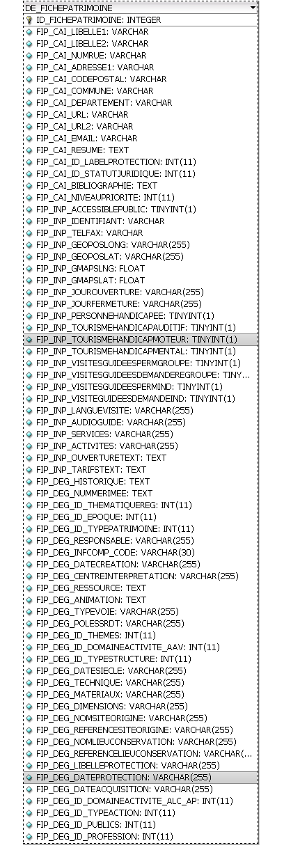
It made SELECT statements easier to write, since you didn't need to remember a dozen table names, but there was little to tell one column apart from another. A developer could think they're selecting the FirstName column for Users, but it could be for Clients if they read the column name too quickly.
Guillaume left the BastilleCo revolution shortly after.
[Advertisement] BuildMaster 4.1 has arrived! Check out the new Script Repository feature and see how you can deploy builds from TFS (and other CI) to your own servers, the cloud, and more.
07 Jul 18:30
[Advertisement] Have you seen BuildMaster 4.3 yet? Lots of new features to make continuous delivery even easier; deploy builds from TeamCity (and other CI) to your own servers, the cloud, and more.

CodeSOD: The Name of the Rows
by Dan Adams-Jacobson
When teams of enterprise software developers are cloistered away from the real world for long enough, an attitude of monasticism prevails. The fragile and fleeting concerns of mortal time fall away, and the developer's mind awakens to the greater, eternal truths that wait unsullied in everlasting Empyrean majesty. Into such a team Cory came, and, under the rigorous guidance of Brother Architect, he learned that only adherence to the Database Schema Commandments could free his soul to bask in the light of the divine.
And, lo, the First Commandment was: Thou shalt name each table having a foreign-key relationship with another table such that the name of the table having the primary key is included in the related table's name.
Since Brother Architect acknowledged that verily the wording of the First Commandment left it open to heretical interpretation, he provided, in his wisdom, the following example tables:
CountryTable
AddressTable
AddressCountryTable -- Foreign keys to AddressTable and CountryTable
And, lo, the Second Commandment was: Thou shalt name each stored procedure whose purpose is to retrieve a particular relation such that the name of the procedure includes both the name of the relation being retrieved and the name of the field or fields used to retrieve it.
Knowing the minds of his fellow monks were still benighted by the manifold temptations of the flesh, Brother Architect provided this clarifying example:
GetAddressCountryByPostcode
Suffused with the wisdom of the Database Schema Commandments, Cory went forth, with Brother Architect's blessing, to make a change to the Controls Automation database. Having completed this work, Cory sinfully amused himself by searching the database for the object with the longest name. Pray pardon him his weakness, friend, and look mirthfully upon his best finding thus far:
GetAutomationExportAutomationExportFieldLUByAutomationExportID
And there was evening, and there was morning—the third normal form.
[Advertisement] Have you seen BuildMaster 4.3 yet? Lots of new features to make continuous delivery even easier; deploy builds from TeamCity (and other CI) to your own servers, the cloud, and more.
07 Jul 18:28
[Advertisement] Have you seen BuildMaster 4.3 yet? Lots of new features to make continuous delivery even easier; deploy builds from TeamCity (and other CI) to your own servers, the cloud, and more.

The Five Alarm Meeting
by Remy Porter
Leigh didn’t have anything to do with automating operations at their NOC, although he was mostly glad it had been done. The system was a bit of a mess, with home-grown programs and scripts sitting atop purchased monitoring packages and a CMDB. It was cumbersome, sometimes spit out incomprehensible and nonsense errors, but it mostly worked, and it saved them a huge amount of time.
It was also critical to their operations. Without these tools, without the scripts and the custom database back end, without the intermediary applications and the nice little stop-light dashboard that the managers could see if they hit refresh five times, nothing could get done. Unfortunately, this utopia covered up a dark underbelly.
We’re going to need a meeting
The operations team were the end users of the software, but they mostly relied on the development team to build it and maintain it. The development team relied on the database team. Once, Leigh needed them to expand the size of a single text field in the database from 25 characters to 50 characters. The development team had no problem updating their applications, but the database team wasn’t ready to start changing column sizes right away. Burt, the head of the database team had to start with a 1-hour meeting with his entire team to discuss the implications. Then he had to have another meeting with the development and operations managers. Then Leigh needed to sit down with the DBAs and justify the extra 25 characters (“That’s a 100% increase in the size of the field!” Burt proclaimed). After 200 man hours, the field was changed.
After the database had been in use for some time, performance started to degrade . Leigh helpfully suggested building an index around some of their frequently executed queries. This small pebble triggered an avalanche of meeting requests. Burt wasn’t about to waste a bunch of hard disk space on an index, just because his customer, the developers, and his own DBAs said so. Over thirty meetings were held before Burt grudgingly agreed to allow one index on a few key fields.
The worst day, however, was the day the database went down, at 8AM on the last Friday of the month. Everything the operations team did ground to a complete and total halt. This had cascading effects down the line to application after application, especially the payroll process which needed to ship a gigantic flat-file to the payroll company so that employee would get their checks that month. Every cellphone in the building started beeping out the clarion call of complete disaster as emergency alert after emergency alert went out. The problem went from “solvable crisis” to “full meltdown panic my hair is on fire” in the space of 15 minutes.
Leigh, keeping his cool, started calling DBAs. Not a one answered their phone. Leigh called Burt directly, again with no answer. Leigh’s boss called Burt’s boss, who swore Burt was available, and that he would be found. Leigh texted, emailed, IMed, and stalked the halls, hoping to find one lone DBA that could look at the database. At the end of the first hour, every middle manager in the building was in the hunt. At the end of the second hour, most of upper management had joined them.
The database remained stubbornly down, with it, most of the network operations were shut down.
And then the DBAs reappeared on IM. The underlying problem was a full transaction log, which was solved in moments with a log rotation. Operations resumed. Leigh, however, was curious. He pinged Sally, one of the DBAs, and asked where they had been.
“When the database went down,” Sally replied, “Burt called an emergency meeting. He locked us all in a conference room and didn’t let anyone leave until we had a ‘plan of action’. We weren’t even allowed bathroom breaks!”
[Advertisement] Have you seen BuildMaster 4.3 yet? Lots of new features to make continuous delivery even easier; deploy builds from TeamCity (and other CI) to your own servers, the cloud, and more.
byron lewis, Ronald.phillips and one other like this
07 Jul 18:21
[Advertisement] Have you seen BuildMaster 4.3 yet? Lots of new features to make continuous delivery even easier; deploy builds from TeamCity (and other CI) to your own servers, the cloud, and more.

The System
by snoofle
One of J.W.'s clients called him in to help diagnose and fix some reliability problems with the deployment system. The client was a small shop of about ten developers, one dual-role QA/manager, one SA who controlled the QA and production machines, and the requisite bean counters.
Upon arrival, J.W. was proudly shown the home-grown system that the manager had cobbled together. The developers would fill out a wiki page template for each release. The template had a section for:
- Configurations
- Database
- Network
- Hardware
- System Software (e.g. web servers, etc.)
- Application
- Miscellaneous
- List of approvers for each section, as well as the whole release
Each relevant section for a given release had a descriptive paragraph containing the purpose and scope of the change, and a list of the affected files. It also had a section where the developers would put the exact (*nix) commands that had to be used to accomplish the task.
For such a small shop, the procedures seemed fairly solid. Everything had to be built and pass assorted tests and code reviews in development. The SA would perform the exact deployment steps on the QA machines. The manager would put on his QA hat and test everything. The SA would then repeat the deployment process on the production machines, using the exact same commands that had been tested in both development and QA. Finally, the manager would test everything in production.
So what sort of problems were occurring? It turned out that no matter how meticulously the developers had scripted the deployment tasks, things always seemed to go wrong, randomly, in deployments to both QA and production. Even things that worked perfectly while deploying to QA would break during deployments to production, and never twice in the same way or place.
After watching them go through the motions of a release, the developers seemed to be following the procedures correctly and according to plan. The wiki page for each release looked fine to the naked eye.
While loading the deployment wiki page, J.W. happened to notice that there was image alt-text appearing briefly before the script text would appear. But why would there be alt-text where simple text should be?
A quick view-page-source turned up the culprit. The manager wanted to make sure that nobody changed the instructions after they were posted, so he had the developers write up the script text, verify that it worked, then take a screen shot of it and put the image of the script on the wiki page.
The poor SA, somewhat afraid of making a typo while transcribing potentially long sequences of complex commands and data, decided to mitigate the risk by automating the task. How was this feat accomplished? The manager decided that the SA would run OCR on the images of the scripts and data. The SA would then run the output of the OCR.
Of course, the OCR would occasionally frequently misread something and hilarity would ensue.
J. W. explained the folly of all of this to the manager and explained that perhaps simply putting the text of the commands themselves on the Wiki would solve the problem. Unfortunately, the manager insisted that the scripts needed to be protected from unauthorized changes, and using images of them was the only way to do just that...
  JW:  OCR is not reliable enough to do this; that's why you're having all the problems
  SA:  Agreed, but manually typing in large quantities of data and commands is far less reliable
  Mgr: Then the solution is to check the output of the OCR before using it
  JW:  And how do you propose to do that?
  Mgr: Simple: after the OCR is performed, you will run a script to compare it to the scripts in source control
  JW:  Why not just use the scripts directly from source control instead of the OCR?
  Mgr: Because the OCR software was a significant expense and is part of the procedure!
And so it went. The SA would perform OCR on the pictures of the scripts. Then he would run diff on the scripts in source control and the output of the OCR, and resolve all differences to match the source script. This would be repeated until there were no differences. Finally, the SA would run the generated file to perform the requisite tasks.
And the manager was proud of the system he had created.
[Advertisement] Have you seen BuildMaster 4.3 yet? Lots of new features to make continuous delivery even easier; deploy builds from TeamCity (and other CI) to your own servers, the cloud, and more.
byron lewis likes this
07 Jul 18:15
[Advertisement] Have you seen BuildMaster 4.3 yet? Lots of new features to make continuous delivery even easier; deploy builds from TeamCity (and other CI) to your own servers, the cloud, and more.

Scriptzilla
by Charles Robinson
In the late 90s, Jeremy fought a battle against a menace more terrifying than the dreaded Y2K bug. He maintained a network management application running on Solaris which managed TDM and ATM switches, called PortLog. This prototype CMDB maintained a database of all of the equipment in the network. It created a unique identifier encoded each device’s shelf, slot and port number according to a “magic” formula. That formula needed to change in the next release, thus forcing the unique ID of each device to change as well, in every deployed instance of their database.

Ross, Jeremy’s boss and PortLog guru, provided Jeremy an update script to guide this conversion. One client volunteered to be a -guinea pig- pilot site. With appropriate permission in writing, Jeremy kicked the script off, expecting it to take 20 minutes tops. Surely just converting a bunch of numbers couldn’t take much longer than that, right? But Ross’ script kept running. And running. And…
…
…
…
running.
12 whole hours and a few cans of energy drink later, the script finally reported a successful completion. The pilot site was small, and took 12 hours to convert. How long would their much larger clients take? 12 hours of downtime wasn’t acceptable, and it was only going to get worse.
Jeremy poked through the database and found all the ID’s had been updated, but several of them had the same number, thus defeating the purpose of an ID field in the first place. Out of morbid curiosity, he cracked open Ross’ script to see what the hell it was doing. A MASSIVE stored procedure stared back at him like Godzilla peering through the window of a high-rise. Inside the procedure, there were foreach loops - one per table, once per piece of equipment. Inside all foreach loops, the key step looked like:
ON EXCEPTION
  UPDATE <table> SET adp_no=<new value> WHERE …; --this fixes the duplicate key exception. Runs much faster now! - Ross
END EXCEPTION WITH RESUME;
It did indeed “fix” the duplicate key exception, by forcing the value to be set whenever any exception was thrown, including a duplicate key violation. Ross didn’t care that the equipment IDs ceased to be unique. And this made it “much faster”?
Jeremy paid Ross a visit. As diplomatically as possible, Jeremy explained to him everything that was wrong with the script, and how a much more reliable, efficient one could be created before their go-live date. The new script would be much shorter, easier to support, run in minutes, and most important: actually work. Ross, of course, wasn’t having any of it.
“No way, Jeremy!” Ross bellowed back at him. “It’s too late in the game to be throwing unknown stuff at this. My script has been tested and proven to work. You said yourself that it said ‘successful’ after it was done running. That means it works!”
“Ross, this thing took 12 whole hours to run for a medium-sized client, and the data wasn’t even right…” Jeremy pleaded. “If you’d just let me…”
“It printed ‘successful’! It wouldn’t have done that if it didn’t work!” Ross interrupted. He took a few moments to catch his breath, and then found the diplomatic solution: "I’m not perfect, but since you are, you can take my existing, TESTED script and modify it. Making something from scratch is out of the question in this time-frame so get started!
Jeremy slinked back to his desk and pondered his existence. Then a light bulb burst to life over his head. He could still make the quick, simple efficient script he wanted to and just Modify Ross’ script to call it and exit immediately. All of Ross’s code would still be there, so if Ross did a cursory examination of the script, nothing would look wrong. Since Ross rarely actually did the production releases, he’d never catch on.
The next weekend, Jeremy and his fellow engineers were prepared to assault their largest client’s data with the mean script he came up with. “Are we going to be here all weekend? I heard Ross’ conversion script took 12 hours for the pilot site.” a colleague asked.
“Don’t worry, I got this!” Jeremy said confidently. “I… um… tuned Ross’s script. But, ah… let’s keep this our little secret though because if Ross finds out how lean this monster can really be, his insecurity will boil over into rage.”
They were done with their work and out at the pub before sundown. Jeremy left an email for Ross to find Monday telling him how the minor tweaks he made to the script paid off, but of course Ross deserved most of the credit. Scriptzilla had been tamed, but the code remained in the script, like Godzilla lurking beneath the sea. Jeremy feared that it would one day rise again…
[Advertisement] Have you seen BuildMaster 4.3 yet? Lots of new features to make continuous delivery even easier; deploy builds from TeamCity (and other CI) to your own servers, the cloud, and more.
byron lewis, Ronald.phillips likes this
07 Jul 17:48

Miscellaneous Notes on the PASS NomCom and General Election
by Andy Warren
Interesting day yesterday. A spirited discussion on Twitter, a challenging post from candidate Mark Broadbent, and a couple good threads on the NomCom discussion forum. I’ve picked some of the points where I want to add a few notes of my own (I’m not speaking for PASS on any of these, and in most cases my direct knowledge of some of this is now a couple years old). Most of these are complex topics worth a deeper discussion.
Nomcom Ranking
The NomCom ranks all candidates that are qualified (meets the minimum criteria as described in the voting process). The ranking does at least four things:
- Tries to make a very subjective process a little less subjective
- Rankings are used if we have too many candidates (current rules call for a limit of 3 candidates per seat available, you’ll often hear me call it 3x)
- Rankings are a way to communicate to candidates how they did in a way that is informative and as polite as possible, so they can decide if they want to continue or withdraw (the default is continue). Imagine there are 9 candidates and you placed 9th. If you’re within a point or two of the leader you will certainly continue, but what if you’re 10 points down? You might decide to withdraw, work on some things, and come back in a later election. The point here is not to force people out, merely to treat them with respect and courtesy. If someone cares enough to run but doesn’t have (and possibly doesn’t realize) the skills and experience they are missing it could wind up being a painful or embarrassing experience for them. I know of one instance where a candidate withdrew because of that and that person felt like it was the right thing to do.
- Finally, for voters who have a hard time figuring out style from substance, they can look at the ratings as a way to see what a very serious and informed group think of the candidates in aggregate. In fact, candidates are listed on the ballot by order of ranking.
I like this system.
Voting Password Security
Brent Ozar raised the question about how credentials were transferred to Simple Voting. It’s a very good question, pains me that I never asked way back when about the security. As far as I know sqlpass.org still runs on DNN and whether credentials are stored in clear text depends on the configuration. There doesn’t seem to be any SSL in use or available, that’s not promising. Troy Hunt, care to come take a look? The question deserves an answer, and certainly the SSL issue needs to be addressed.
Voter Turnout
In the spirit of transparency and dashboarding PASS has the chart below posted at http://www.sqlpass.org/Elections/Archive.aspx (thanks to Gavin Campbell for finding it). What it doesn’t show unfortunately is the number of valid/registered voters, the closest is this link http://www.sqlpass.org/AboutPASS.aspx that references more than 100k members. 1500 votes out of 100,000 doesn’t look great. The challenge is that many of those 100k joined by attending SQLSaturday (a decision I agree with) and that list probably includes members back to the beginning of PASS. In previous years PASS has deduped the voting list, I’m not sure it deduped the member list – many of us have ended on the list with multiple email addresses. It has made an effort this year to determine eligible voters based on having updated their profile (not great at all, but better than nothing). There is the mailing list, then there is the voting list (deduped/qualified), and then of that there is some number of members that are interested and have time to vote. I’d like to see PASS post the count for the voting list each year to go this chart as well (and maybe even a regional break down). Does PASS do enough to encourage voting? I think there is always more that can be done, but anyone interested enough to read the Connector certainly should see it happening. Is it easy to vote? Arguably it’s harder this year than last year because you have to find/remember your PASS login (last year each voter got a unique link good for one vote, no password required), but it’s nothing that will take more than a couple minutes. Is it a conspiracy? No, sadly no conspiracy here! Why don’t more people vote? Go to any Chapter meeting and you’ll see why – as much as Chapter leaders try to make the connection, Chapters (and SQLSaturday) are local, and more than that, they often feel like they don’t know enough to cast an informed vote, and I suspect – I’m guessing – for many the inside baseball of PASS just doesn’t hit the Top 10 things they care about. Should we work on it? Yes. All of it. But the number that we should measure, because we have it, is the turnout. Why did it drop last year? Can we grow it this year? As much as I want it to grow, I want it to be solid growth, people that vote because they care, because they want some kind of change, not to hit a quota of votes per Chapter or per state.

Should We Campaign For the NomCom?
First, the rules clearly allow it. Beyond that, what’s our goal? I believe we want a fair, experienced, diverse NomCom that will follow the charter given to them by the Board. We’ve got candidates, how do we discern between them? The NomCom app is trivial, and I’m not opposed to that (the app for Board candidates is quite a bit more strenuous) and we like that because we don’t want to put too many barriers in place – the NomCom is hard work. We could add more to the application, but then you’re only getting things that PASS cares about, which may not be the things you care about. How we campaign is interesting. I elected (so to speak) to put up a blog post about running, because I write about professional things I do, that gets a quick tweet (because it does it when I post), and I answered the questions posted on the discussion forum for the election. Beyond that, the discussion on Twitter was relevant and I’d have been in that even if I wasn’t a candidate, time permitting. This post – campaigning? Maybe, it’s more I want to share what I know/think, with equal chances it helps/hurts in the election. I don’t want complicated elections or campaigns, but I think a campaign is a good way to see who has game. The NomCom election is a way for people to get their feet wet. Shorter, milder, it’s a good way to learn the process, get some ideas, meet some people, and still do some good.
International Representation
I’ll admit to being less than zoomed in on this. I like that PASS is growing to be the international org it has said it was (or wanted to be), and I think that journey takes time. Would changing the allocation for the NomCom be a step in the right direction. I’m stuck at maybe. At some point it should be proportional OR we should change so that there is a PASS World Org, then PASS North America, PASS Europe, or even PASS UK. I think that is a decision we’re not there on, at least from what I’ve seen. I’d love to see the Board talk more about the roadmap, then we could se if the NomCom allocation is a miss, or just not there according to the Roadmap
NomCom Charter
The ERC (election review component) of the NomCom this year remains to be seen. I have huge concerns about one group trying to do two tasks, when clearly the primary task is to vet and pick the slate. I’d like to see the Board publish the charter and ideally would have done so before the election. My hope is that the committee generates a lot of notes and makes suggestions, but then that is followed by Board review and/or a mini to full ERC as seems to be needed.
07 Jul 17:46
SQL Server 2014: Using New Cardinality Estimator for databases created in lower version
by prince rastogi
Hi Friends,
In our previous blog we have seen how we can use new cardinality Estimator for newly created databases under SQL Server 2014.Link for that blog is mentioned below:
Today we will see about how we can use New Cardinality Estimator for databases created under previous version of SQL Server. The logic is very simple here, from previous post we know that New Cardinality estimator can be used if database is having compatibility level 120. That means if you have migrated your database from previous version of SQL Server to SQL Server 2014 and you want to use New Cardinality Estimator then you have to change the compatibility level of that database to 120. Let me show you this thing practically.
I have created one new database under SQL Server 2012. I have restored the backup of this database to SQL server 2014 instance. As of now the compatibility level of this database is 110. You can check this by using below query:
Select compatibility_level from sys.databases where name='CETEST'
![]()
Now from Query Plan you can see that as of now this database is using Old version of Cardinality Estimator. [Here it will not show you version details]
SELECT TOP 1 * FROM [xtTest]


Now if you want to use new cardinality estimator then change the compatibility level of that database by using below query:
USE [master]
GO
ALTER DATABASE [CETEST] SET COMPATIBILITY_LEVEL = 120
GO
Select compatibility_level from sys.databases where name='CETEST'
![]()
After changing compatibility level, now you can check which version of cardinality estimator is in use now:
USE [CETEST]
GO
SELECT TOP 1 * FROM [xtTest]
Now run the above query along with actual execution plan. Right click on left most operators in plan and click on properties:

From above property window, it is clear that we can use new cardinality estimator for databases created in lower versions by restoring them to SQL Server 2014 and changing compatibility mode to 120.
HAPPY LEARNING!
If you liked the post, do like us on FaceBook at http://www.facebook.com/SQLServerGeeks
Have a SQL Server question? Join the fastest growing SQL Server group on FaceBook - http://www.facebook.com/groups/458103987564477/
Thanks & Regards:
Prince Kumar Rastogi
07 Jul 17:45
TPC-H Benchmarks on SQL Server 2014 with Columnstore
by jchang
Three TPC-H benchmark results were published in April of this year at SQL Server 2014 launch, where the new updateable columnstore feature was used. SQL Server 2012 had non-updateable columnstore that required the base table to exist in rowstore form....(read more)
07 Jul 17:44

SQL 2014 does data the way developers want
by Rob Farley
A post I’ve been meaning to write for a while, good that it fits with this month’s T-SQL Tuesday, hosted by Joey D’Antoni ( @jdanton)
Ever since I got into databases, I’ve been a fan. I studied Pure Maths at university (as well as Computer Science), and am very comfortable with Set Theory, which undergirds relational database concepts. But I’ve also spent a long time as a developer, and appreciate that that databases don’t exactly fit within the stuff I learned in my first year of uni, particularly the “Algorithms and Data Structures” subject, in which we studied concepts like linked lists. Writing in languages like C, we used pointers to quickly move around data, without a database in sight. Of course, if we had a power failure all this data was lost, as it was only persisted in RAM. Perhaps it’s why I’m a fan of database internals, of indexes, latches, execution plans, and so on – the developer in me wants to be reassured that we’re getting to the data as efficiently as possible.
Back when SQL Server 2005 was approaching, one of the big stories was around CLR. Many were saying that T-SQL stored procedures would be a thing of the past because we now had CLR, and that obviously going to be much faster than using the abstracted T-SQL. Around the same time, we were seeing technologies like Linq-to-SQL produce poor T-SQL equivalents, and developers had had a gutful. They wanted to move away from T-SQL, having lost trust in it. I was never one of those developers, because I’d looked under the covers and knew that despite being abstracted, T-SQL was still a good way of getting to data. It worked for me, appealing to both my Set Theory side and my Developer side.
CLR hasn’t exactly become the default option for stored procedures, although there are plenty of situations where it can be useful for getting faster performance.
SQL Server 2014 is different though, through Hekaton – its In-Memory OLTP environment.
When you create a table using Hekaton (that is, a memory-optimized one), the table you create is the kind of thing you’d’ve made as a developer. It creates code in C leveraging structs and pointers and arrays, which it compiles into fast code. When you insert data into it, it creates a new instance of a struct in memory, and adds it to an array. When the insert is committed, a small write is made to the transaction to make sure it’s durable, but none of the locking and latching behaviour that typifies transactional systems is needed. Indexes are done using hashes and using bw-trees (which avoid locking through the use of pointers) and by handling each updates as a delete-and-insert.
This is data the way that developers do it when they’re coding for performance – the way I was taught at university before I learned about databases. Being done in C, it compiles to very quick code, and although these tables don’t support every feature that regular SQL tables do, this is still an excellent direction that has been taken.
07 Jul 17:44
SQL Server High Availability and Disaster Recovery Options
by Tim Radney
Working with Microsoft SQL Server for many years I have spent a lot of time discussing the importance of the availability of SQL Server databases. Questions that always come up when discussing availability of the data is “Recovery Time Objective – RTO” and “Recovery Point Objective – RPO”. Both questions are very important when determining your solution for high availability (HA) within your data center as well as your solution for disaster recovery (DR).
Microsoft SQL Server gives us several options for mitigating potential risk for our SQL Server environments. Each solution has its pros and cons and careful consideration should go into your solution. Before you can build a solution you have to have requirements on what risk you are trying to protect against. Some items you might want to protect against are OS failure, hardware failure, data corruption, or a data center failure. We have different options to help mitigate these potential failures and each solution comes with a certain cost and level of complexity. For organizations, they have to weigh the cost of the solution and complexity to manage it against the actual risk. I like to say that it comes down to a math problem that usually involves a budget. What are some technologies we typically see implemented to address HA/DR with SQL Server? Below you will see a chart I like to use that demonstrates some of the pros and cons of Log Shipping, Database Mirroring, Replication, Windows Failover Clusters, Availability Groups, and Virtualization (not a SQL technology) 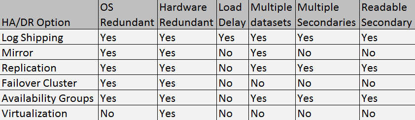
Many times when discussing HA and DR people tend to confuse or mix the two. HA is a system designed that allows for minimal downtime, typically this is for protection from an OS or hardware failure. DR is risk avoidance on a much larger scale. When discussing DR we typically cover risk management, RPO, RTO and build a disaster recovery plan. DR typically involves a second data center whereas HA is typically building redundancy within your data center.
As you can see from the list above, all but virtualization provide both hardware and OS level protection. Log Shipping is the only solution that provides a load delay in synchronizing data. This is a very important feature that can help you protect against an accidental data oops. Imagine ingesting bad that would require you to restore a database, or have an accident where an update/delete statement was ran without a where clause. If you were using replication, mirroring or any other HA solution that provides near real time replication, those transactions would also be applied against your replica. If you had a load delay of 12 to 24 hours you could roll the logs to just before the accident and be back online much quicker than restoring the database.
As previously stated, in order to know which solution is best for you, you really have to know what your requirements are. For me, I typically use a combination of most of the solutions depending on my environment. I have a combination of log shipping, failover clustering, availability groups and virtualization in place. For very large critical environments, a log shipped secondary provides a nice level of comfort knowing I can bring a multi terabyte database back online in minutes in the event I have a data issue.
![]()
07 Jul 17:39
Fixes for SQL Server 2012 & 2014 Online Index Rebuild Issue
by Aaron Bertrand
There is a regression bug in SQL Server 2012 and SQL Server 2014 where, if you rebuild an index online in parallel, and you also experience a fatal error such as a lock timeout, you could experience data loss or corruption. This should be a relatively rare scenario (Phil Brammer has a simple repro in Connect #795134), but data loss is data loss, and I am not prepared to gamble. The fix is described in KB #2969896 : FIX: Data loss in clustered index occurs when you run online build index in SQL Server 2012.
Not everyone needs to be concerned about this issue. If you are not running Enterprise (or an equivalent) Edition, you can't perform parallel or online rebuilds in the first place (and there are probably some folks on Enterprise not rebuilding or not rebuilding online). If you have instance-wide MAXDOP set to 1, they can't go parallel unless you override it at the statement level. But, if you are on 2012 or 2014, running an adequate edition, and your online rebuilds could go parallel, you are vulnerable to this problem.
As I alluded to above, this problem could manifest in SQL Server 2012 RTM, Service Pack 1, and even Service Pack 2, which was released on June 10. The bug was not fixed until long after the SP2 code was frozen, so SP2 does not include this fix or any of the fixes from SP1 CU #10 or #11. I blogged about this here. The RTM branch is officially out of support, so you will not be seeing a fix there. The issue can also occur in SQL Server 2014.
There are now cumulative updates available for SQL Server 2012 Service Pack 1 & 2 as well as SQL Server 2014. A quick summary of the options I recommend:
If your branch / @@VERSION is…
|
…you should… | |||||||
|---|---|---|---|---|---|---|---|---|
| SQL Server 2012 RTM | 11.0.2100 -> 11.0.2999 |
|
||||||
| SQL Server 2012 Service Pack 1 | 11.0.3000 -> 11.0.3436 |
|
||||||
| 11.0.3437 -> 11.0.5057 | Do nothing; you already have the fix. | |||||||
| SQL Server 2012 Service Pack 2 | 11.0.5058 – > 11.0.5521 |
|
||||||
| 11.0.5522 or greater | Do nothing; you already have the fix. | |||||||
| SQL Server 2014 RTM | 12.0.2000 – > 12.0.2369 |
|
||||||
| 12.0.2370 or greater | Do nothing; you already have the fix. | |||||||
| * If you install the SP1 hotfix or Cumulative Update #11 and then install SP2, you will undo those changes, including this fix. | ||||||||
Solutions for the hotfix/CU averse
Since all affected branches (well, except 2012 RTM) have an on-demand hotfix and/or a cumulative update that addresses the issue, the easy answer is to just install the relevant update. However, you may be in a scenario where your company policy or testing cycles prevent you from deploying these updates quickly, or maybe ever. So what other options do you have?
- You can stop performing rebuilds until there is a new service pack available for your branch (maybe you can just stick with
REORGANIZEfor now). Unfortunately, if you are in a "service pack only" company, your options are very limited: you can fight harder to change that policy, or you can wait for SQL Server 2012 Service Pack 3 (which may be a long time, or may simply never come – see FAQ #21 here) or SQL Server 2014 Service Pack 1 (which we probably won't see before 2015 rolls around). - You can set the instance-wide
max degree of parallelismto 1, however this may have a negative effect on the rest of your workload – think about things like multi-threaded DBCC, parallel queries against or between partitioned tables, and other operations where you may want to reduce parallelism but not eliminate it altogether. Also, this setting won't affect an online rebuild with, say, an explicitMAXDOP = 8hard-coded into the command, as this will override thesp_configuresetting.
- You can add the
WITH (MAXDOP = 1)option manually to all of your rebuild commands. (Note: you don't have to do this for XML indexes, since they inherently run single-threaded, but I would just apply it to all rebuilds for consistency and to avoid any unnecessary conditional logic.)
- You can set your index maintenance jobs to run as a specific login, and then use Resource Governor to create a Workload Group that limits that login's
MAX_DOPto 1, regardless of what they are doing. I have an example of this in the 2008 white paper I wrote with Boris Baryshnikov, Using the Resource Governor, in the section entitled, "Limiting Parallelism for Intensive Background Jobs."
- If you are using Ola Hallengren's index maintenance solution, you can add the
@MaxDopparameter to your calls todbo.IndexOptimize:
EXEC dbo.IndexOptimize /* other parameters */ @MaxDop = 1; - If you are using SQL Sentry Fragmentation Manager, you can dictate the level of
MAXDOPto use under Settings – and you can do this enterprise-wide, per instance, per database, or even per individual index (in this case, you'd probably want to set this per instance, for all instances without a fix available):

Fragmentation Manager settings for the instance (left) and an individual index (right). - If you're using Maintenance Plans for your index rebuilds, you're going to have to change them to use Execute T-SQL Statement Tasks, and write your
ALTER INDEX ... WITH (ONLINE = ON, MAXDOP = 1);commands manually (so may as well switch to an automated solution). See, the Index Rebuild Task does not have an exposed property forMAXDOP, even though it has been requested multiple times (most recently in 2012, by Alberto Morillo, and as far back as 2006, by Linchi Shea). And just look at all of these other useful properties they expose, likeAdvSortInTempdb,ObjectTypeSelection, andTaskAllowesDatbaseSelection[sic2!]:

All those options, but still no cure for MAXDOP.The post Fixes for SQL Server 2012 & 2014 Online Index Rebuild Issue appeared first on SQLPerformance.com.
Sergey likes this
07 Jul 17:38

Using SQL Server in Microsoft Azure Virtual Machine? Then you need to read this…
by psssql
Over the past few months we noticed some of our customers struggling with optimizing performance when running SQL Server in a Microsoft Azure Virtual Machine, specifically around the topic of I/O Performance.
We researched this problem further, did a bunch of testing, and discussed the topic at length among several of us in CSS, the SQL Server Product team, the Azure Customer Advisory Team (CAT), and the Azure Storage team.
Based on that research, we have revised some of the guidelines and best practices on how to best configure SQL Server in this environment. You can find this collective advice which includes a quick “checklist” at this location on the web:
http://msdn.microsoft.com/en-us/library/azure/dn133149.aspx
If you are running SQL Server already in Microsoft Azure Virtual Machine or making plans to do so, I highly encourage you to read over these guidelines and best practices.
There is other great advice in our documentation that covers more than just Performance Considerations. You can find all of these at this location:
http://msdn.microsoft.com/en-us/library/azure/jj823132.aspx
If you deploy any of these recommendations and find they are not useful, cause you problems. or are not effective, I want to hear from you. Please contact me at bobward@microsoft.com with your experiences
Bob Ward
Microsoft
.
07 Jul 17:38
Dirty Secrets of the CASE Expression
by Aaron Bertrand
The CASE expression is one of my favorite constructs in T-SQL. It is quite flexible, and is sometimes the only way to control the order in which SQL Server will evaluate predicates.
However, it is often misunderstood. Not surprisingly, I have a few examples.
CASE is an expression, not a statement
Likely not important to most people, and perhaps this is just my pedantic side, but a lot of people call it a CASE statement – including Microsoft, whose documentation uses statement and expression interchangeably at times. I find this mildly annoying (like row/record and column/field), and it's mostly semantics, but there is an important distinction: an expression returns a result. When people think of CASE as a statement, it leads to experiments in code shortening like this:
SELECT CASE [status]
    WHEN 'A' THEN
        StatusLabel      = 'Authorized',
        LastEvent        = AuthorizedTime
    WHEN 'C' THEN
        StatusLabel      = 'Completed',
        LastEvent        = CompletedTime
    END
FROM dbo.some_table;
This type of control-of-flow logic may be possible with CASE statements in other languages (like VBScript), but not in Transact-SQL's CASE expression. To use CASE within the same query logic, you would have to use a CASE expression for each output column:
SELECT
  StatusLabel = CASE [status]
      WHEN 'A' THEN 'Authorized'
      WHEN 'C' THEN 'Completed' END,
  LastEvent = CASE [status]
      WHEN 'A' THEN AuthorizedTime
      WHEN 'C' THEN CompletedTime END
FROM dbo.some_table;
CASE will not always short circuit
The official documentation implies that the entire expression will short-circuit, meaning it will evaluate the expression from left-to-right, and stop evaluating when it hits a match:
The CASE statement [sic!] evaluates its conditions sequentially and stops with the first condition whose condition is satisfied.
However, this isn't always true. And to its credit, at least in the 2014 docs, the page goes on to try to explain one scenario where this isn't guaranteed. But it only gets part of the story:
In some situations, an expression is evaluated before a CASE statement [sic!] receives the results of the expression as its input. Errors in evaluating these expressions are possible. Aggregate expressions that appear in WHEN arguments to a CASE statement [sic!] are evaluated first, then provided to the CASE statement [sic!]. For example, the following query produces a divide by zero error when producing the value of the MAX aggregate. This occurs prior to evaluating the CASE expression.
The divide by zero example is pretty easy to reproduce, and I demonstrated it in this answer on dba.stackexchange.com:
DECLARE @i INT = 1;
SELECT CASE WHEN @i = 1 THEN 1 ELSE MIN(1/0) END;
Result:
Msg 8134, Level 16, State 1
Divide by zero error encountered.
Divide by zero error encountered.
There are trivial workarounds (such as ELSE (SELECT MIN(1/0)) END), but this comes as a real surprise to many who haven't memorized the above sentences from Books Online. I was first made aware of this specific scenario in a conversation on a private e-mail distribution list by Itzik Ben-Gan (@ItzikBenGan), who in turn was initially notified by Jaime Lafargue. I reported the bug in Connect #690017 : CASE / COALESCE won't always evaluate in textual order; it was swiftly closed as "By Design." Paul White (blog | @SQL_Kiwi) subsequently filed Connect #691535 : Aggregates Don't Follow the Semantics Of CASE, and it was closed as "Fixed." The fix, in this case, was clarification in the Books Online article; namely, the snippet I copied above.
This behavior can yield itself in some other, less obvious scenarios, too. For example, Connect #780132 : FREETEXT() does not honor order of evaluation in CASE statements (no aggregates involved) shows that, well, CASE evaluation order is not guaranteed to be left-to-right when using certain full-text functions either. On that item, Paul White commented that he also observed something similar using the new LAG() function introduced in SQL Server 2012. I don't have a repro handy, but I do believe him, and I don't think we've unearthed all of the edge cases where this may occur.
So, when aggregates or non-native services like Full-Text Search are involved, please do not make any assumptions about short circuiting in a CASE expression.
Expressions can be evaluated more than once
I often see people writing a simple CASE expression, like this:
SELECT CASE @variable
  WHEN 1 THEN 'foo'
  WHEN 2 THEN 'bar'
END
It is important to understand that this will actually be executed as a searched CASE expression, like this:
SELECT CASE
  WHEN @variable = 1 THEN 'foo'
  WHEN @variable = 2 THEN 'bar'
END
The reason it is important to understand that the expression being evaluated will actually be referenced multiple times, is because it can actually be evaluated multiple times. When this is a variable, or a constant, or a column reference, this is unlikely to be a real problem; however, things can change quickly when it's a non-deterministic function. Consider that this expression yields a SMALLINT between 1 and 3; go ahead and run it many times, and you will always get one of those three values:
SELECT CONVERT(SMALLINT, 1+RAND()*3);
Now, put this into a simple CASE expression, and run it a dozen times – eventually you will get a result of NULL:
SELECT [result] = CASE CONVERT(SMALLINT, 1+RAND()*3)
  WHEN 1 THEN 'one'
  WHEN 2 THEN 'two'
  WHEN 3 THEN 'three'
END;
How does this happen? Well, the entire CASE expression is actually expanded to a searched expression, as follows:
SELECT [result] = CASE
  WHEN CONVERT(SMALLINT, 1+RAND())*3 = 1 THEN 'one'
  WHEN CONVERT(SMALLINT, 1+RAND())*3 = 2 THEN 'two'
  WHEN CONVERT(SMALLINT, 1+RAND())*3 = 3 THEN 'three'
  ELSE NULL -- this is always implicitly there
END;
So, what happens is that each WHEN clause evaluates and invokes RAND() independently – and in each case it could yield a different value. Let's say we enter the expression, and we check the first WHEN clause, and the result is 3. So we skip that clause and move on. It is conceivable that the next two clauses will both return 1 when RAND() is evaluated again – in which case none of the conditions are evaluated to true, so the ELSE takes over.
This problem is not limited to the RAND() function. Imagine the same style of non-determinism coming from these moving targets:
SELECT
  [crypt_gen]   = 1+ABS(CRYPT_GEN_RANDOM(10) % 20),
  [newid]       = LEFT(NEWID(),2),
  [checksum]    = ABS(CHECKSUM(NEWID())%3);
These expressions can obviously yield a different value if evaluated multiple times. And with a searched CASE expression, there will be times when every re-evaluation happens to fall out of the search specific to the current WHEN, and ultimately hit the ELSE clause. To protect yourself from this, one option is to always hard-code your own explicit ELSE; just be careful about the fallback value you choose to return, because this will have some skew effect if you are looking for even distribution. Another option is to just change the last WHEN clause to ELSE; however this will still lead to uneven distribution. The preferred option, in my opinion, is to try and coerce SQL Server to evaluate the condition once (though this isn't always possible within a single query). For example, compare these two results:
-- Query A: expression referenced directly in CASE; no ELSE:
SELECT x, COUNT(*) FROM
(
  SELECT x = CASE ABS(CHECKSUM(NEWID())%3)
  WHEN 0 THEN '0' WHEN 1 THEN '1' WHEN 2 THEN '2' END
  FROM sys.all_columns
) AS y GROUP BY x;

-- Query B: additional ELSE clause:
SELECT x, COUNT(*) FROM
(
  SELECT x = CASE ABS(CHECKSUM(NEWID())%3)
  WHEN 0 THEN '0' WHEN 1 THEN '1' WHEN 2 THEN '2' ELSE '2' END
  FROM sys.all_columns
) AS y GROUP BY x;

-- Query C: Final WHEN converted to ELSE:
SELECT x, COUNT(*) FROM
(
  SELECT x = CASE ABS(CHECKSUM(NEWID())%3)
  WHEN 0 THEN '0' WHEN 1 THEN '1' ELSE '2' END
  FROM sys.all_columns
) AS y GROUP BY x;

-- Query D: Push evaluation of NEWID() to subquery:
SELECT x, COUNT(*) FROM
(
  SELECT x = CASE x WHEN 0 THEN '0' WHEN 1 THEN '1' WHEN 2 THEN '2' END
  FROM
  (
    SELECT x = ABS(CHECKSUM(NEWID())%3) FROM sys.all_columns
  ) AS x
) AS y GROUP BY x;
Distribution:
| Value | Query A | Query B | Query C | Query D |
|---|---|---|---|---|
| NULL | 2,572 | - | - | - |
| 0 | 2,923 | 2,900 | 2,928 | 2,949 |
| 1 | 1,946 | 1,959 | 1,927 | 2,896 |
| 2 | 1,295 | 3,877 | 3,881 | 2,891 |
Distribution of values with different query techniques
In this case I am relying on the fact that SQL Server chose to evaluate the expression in the subquery and not introduce it to the searched CASE expression, but this is merely to demonstrate that distribution can be coerced to be more even. In reality this may not always be the choice the optimizer makes, so please don't learn from this little trick. :-)
You will observe that if you replace the CHECKSUM(NEWID()) expression with the RAND() expression, you'll get entirely different results; most notably, the latter will only ever return one value. This is because RAND(), like GETDATE() and some other built-in
functions, is given special treatment as a runtime constant, and only evaluated once per reference for the entire row. Note that it can still return NULL just like the first query in the preceding code sample.
This problem is also not limited to the CASE expression; you can see similar behavior with other built-in functions that use the same underlying semantics. For example, CHOOSE is merely syntactic sugar for a more elaborate searched CASE expression, and this will also yield NULL occasionally:
SELECT [choose] = CHOOSE(CONVERT(SMALLINT, 1+RAND()*3),'one','two','three');
IIF() is a function that I expected to fall into this same trap, but this function is really just a searched CASE expression with only two possible outcomes, and no ELSE – so it is tough, without nesting and introducing other functions, to envision a scenario where this can break unexpectedly. While in the simple case it is decent shorthand for CASE, it is also tough to do anything useful with it if you need more than two possible outcomes. :-)
Finally, we should examine that COALESCE can have similar issues. Let's consider that these expressions are equivalent:
SELECT COALESCE(@variable, 'constant');

SELECT CASE WHEN @variable IS NOT NULL THEN @variable ELSE 'constant' END);
In this case, @variable would be evaluated twice (as would any function or subquery, as described in this Connect item).
I was really able to get some puzzled looks when I brought the following example up in a recent forum discussion. Let's say I want to populate a table with a distribution of values from 1-5, but whenever a 3 is encountered, I want to use -1 instead. Not a very real-world scenario, but easy to construct and follow. One way to write this expression is:
SELECT COALESCE(NULLIF(CONVERT(SMALLINT,1+RAND()*5),3),-1);
(In English working from the inside out: convert the result of the expression 1+RAND()*5 to a smallint; if the result of that conversion is 3, set it to NULL; if the result of that is NULL, set it to -1. You could write this with a more verbose CASE expression, but concise seems to be king.)
If you run that a bunch of times, you should see a range of values from 1-5, as well as -1. You will see some instances of 3, and you may have also noticed that you occasionally see NULL, though you might not expect either of those results. Let's check the distribution:
USE tempdb;
GO
CREATE TABLE dbo.dist(TheNumber SMALLINT);
GO
INSERT dbo.dist(TheNumber) SELECT COALESCE(NULLIF(CONVERT(SMALLINT,1+RAND()*5),3),-1);
GO 10000
SELECT TheNumber, occurences = COUNT(*) FROM dbo.dist
  GROUP BY TheNumber ORDER BY TheNumber;
GO
DROP TABLE dbo.dist;
Results (your results will certainly vary, but the basic trend should be similar):
| TheNumber | occurences |
|---|---|
| NULL | 1,654 |
| -1 | 2,002 |
| 1 | 1,290 |
| 2 | 1,266 |
| 3 | 1,287 |
| 4 | 1,251 |
| 5 | 1,250 |
Distribution of TheNumber using COALESCE
Are you scratching your head yet? How do the values NULL and 3 show up, and why is the distribution for NULL and -1 substantially higher? Well, I'll answer the former directly, and invite hypotheses for the latter.
The expression roughly expands to the following, logically, since RAND() is evaluated twice inside NULLIF, and then multiply that by two evaluations for each branch of the COALESCE function. I don't have a debugger handy, so this isn't necessarily *exactly* what is done inside of SQL Server, but it should be equivalent enough to explain the point:
SELECT
  CASE WHEN
      CASE WHEN CONVERT(SMALLINT,1+RAND()*5) = 3 THEN NULL
      ELSE CONVERT(SMALLINT,1+RAND()*5)
      END
    IS NOT NULL
    THEN
      CASE WHEN CONVERT(SMALLINT,1+RAND()*5) = 3 THEN NULL
      ELSE CONVERT(SMALLINT,1+RAND()*5)
      END
    ELSE -1
  END
END
So you can see that being evaluated multiple times can quickly become a Choose Your Own Adventure™ book, and how both NULL and 3 are possible outcomes that don't seem possible when examining the original statement. An interesting side note: this doesn't happen quite the same if you take the above distribution script and replace COALESCE with ISNULL. In that case, there is no possibility for a NULL output; the distribution is roughly as follows:
| TheNumber | occurences |
|---|---|
| -1 | 1,966 |
| 1 | 1,585 |
| 2 | 1,644 |
| 3 | 1,573 |
| 4 | 1,598 |
| 5 | 1,634 |
Distribution of TheNumber using ISNULL
Again, your actual results will certainly vary, but shouldn't by much. The point is that we can still see that 3 falls through the cracks quite often, but ISNULL magically eliminates the potential for NULL to make it all the way through.
I talked about some of the other differences between COALESCE and ISNULL in a tip, entitled "Deciding between COALESCE and ISNULL in SQL Server." When I wrote that, I was heavily in favor of using COALESCE except in the case where the first argument was a subquery (again, due to this bug "feature gap"). Now I'm not so sure I feel as strongly about that.
Simple CASE expressions can become nested over linked servers
One of the few limitations of the CASE expression is that is restricted to 10 nest levels. In this example over on dba.stackexchange.com, Paul White demonstrates (using SQL Sentry Plan Explorer) that a simple expression like this:
SELECT CASE column_name
  WHEN '1' THEN 'a'
  WHEN '2' THEN 'b'
  WHEN '3' THEN 'c'
  ...
END
FROM ...
Gets expanded by the parser to the searched form:
SELECT CASE
  WHEN column_name = '1' THEN 'a'
  WHEN column_name = '2' THEN 'b'
  WHEN column_name = '3' THEN 'c'
  ...
END
FROM ...
But can actually be transmitted over a linked server connection as the following, much more verbose query:
SELECT
  CASE WHEN column_name = '1' THEN 'a' ELSE
    CASE WHEN column_name = '2' THEN 'b' ELSE
      CASE WHEN column_name = '3' THEN 'c' ELSE
      ...
      ELSE NULL
      END
    END
  END
FROM ...
In this situation, even though the original query only had a single CASE expression with 10+ possible outcomes, when sent to the linked server, it had 10+ nested CASE expressions. As such, as you might expect, it returned an error:
Msg 8180, Level 16, State 1
Statement(s) could not be prepared.
Msg 125, Level 15, State 4
Case expressions may only be nested to level 10.
Statement(s) could not be prepared.
Msg 125, Level 15, State 4
Case expressions may only be nested to level 10.
In some cases, you can rewrite it as Paul suggested, with an expression like this (assuming column_name is a string):
SELECT CASE CONVERT(VARCHAR(MAX), SUBSTRING(column_name, 1, 255))
  WHEN 'a' THEN '1'
  WHEN 'b' THEN '2'
  WHEN 'c' THEN '3'
  ...
END
FROM ...
In some cases, only the SUBSTRING may be required to alter the location where the expression is evaluated; in others, only the CONVERT. I did not perform exhaustive testing, but this may have to do with the linked server provider, options like Collation Compatible and Use Remote Collation, and the version of SQL Server at either end of the pipe.
Long story short, it is important to remember that your CASE expression can be re-written for you without warning, and that any workaround you use may later be overruled by the optimizer, even if it works for you now.
Conclusion
I hope I've given some food for thought on some of the lesser-known aspects of the CASE expression, and some insight into situations where CASE – and some of the functions that use the same underlying logic – return unexpected results. Some other interesting scenarios where this type of problem has cropped up:
- Stack Overflow : How does this CASE expression reach the ELSE clause?
- Stack Overflow : CRYPT_GEN_RANDOM() Strange Effects
- Stack Overflow : CHOOSE() Not Working as Intended
- Stack Overflow : CHECKSUM(NewId()) executes multiple times per row
- Connect #350485 : Bug with NEWID() and Table Expressions
The post Dirty Secrets of the CASE Expression appeared first on SQLPerformance.com.
07 Jul 17:37
New Trace Flag to Fix Table Variable Performance
by Aaron Bertrand
It has long been established that table variables with a large number of rows can be problematic, since the optimizer always sees them as having one row. Without a recompile after the table variable has been populated (since before that it is empty), there is no cardinality for the table, and automatic recompiles don't happen because table variables aren't even subject to a recompile threshold. Plans, therefore, are based on a table cardinality of zero, not one, but the minimum is increased to one as Paul White (@SQL_Kiwi) describes in this dba.stackexchange answer.
The way we might typically work around this problem is to add OPTION (RECOMPILE) to the query referencing the table variable, forcing the optimizer to inspect the cardinality of the table variable after it has been populated. To avoid the need to go and manually change every query to add an explicit recompile hint, a new trace flag (2453) has been introduced, but so far only in SQL Server 2012 Service Pack 2:
When trace flag 2453 is active, the optimizer can obtain an accurate picture of table cardinality after the table variable has been created. This can be A Good Thing™ for a lot of queries, but probably not all, and you should be aware of how it works differently from OPTION (RECOMPILE). Most notably, the parameter embedding optimization Paul White talks about in this post occurs under OPTION (RECOMPILE), but not under this new trace flag.
A Simple Test
My initial test consisted of just populating a table variable and selecting from it; this yielded the all-too-familiar estimated row count of 1. Here is the test I ran (and I added the recompile hint to compare):
DBCC TRACEON(2453);

DECLARE @t TABLE(id INT PRIMARY KEY, name SYSNAME NOT NULL UNIQUE);

INSERT @t SELECT TOP (1000) [object_id], name FROM sys.all_objects;

SELECT t.id, t.name
  FROM @t AS t;

SELECT t.id, t.name
  FROM @t AS t OPTION (RECOMPILE);

DBCC TRACEOFF(2453);
Using SQL Sentry Plan Explorer, we can see that the graphical plan for both queries in this case is identical, probably at least in part because this is quite literally a trivial plan:

Graphical plan for a trivial index scan against @t
However, the estimates are not the same. Even though the trace flag is enabled, we still get an estimate of 1 coming out of the index scan if we don't use the recompile hint:

Comparing estimates for a trivial plan in the statements grid

Comparing estimates between trace flag (left) and recompile (right)
If you've ever been around me in person, you can probably picture the face I made at this point. I thought for sure that either the KB article listed the wrong trace flag number, or that I needed some other setting enabled for it to truly be active.
Benjamin Nevarez (@BenjaminNevarez) quickly pointed out to me that I needed to look closer at the "Bugs that are fixed in SQL Server 2012 Service Pack 2" KB article. While they've obscured the text behind a hidden bullet under Highlights > Relational Engine, the fix list article does a slightly better job at describing the behavior of the trace flag than the original article (emphasis mine):
If a table variable is joined with other tables in SQL Server, it may result in slow performance due to inefficient query plan selection because SQL Server does not support statistics or track number of rows in a table variable while compiling a query plan.
So it would appear from this description that the trace flag is only meant to address the issue when the table variable participates in a join. (Why that distinction isn't made in the original article, I have no idea.) But it also works if we make the queries do a little more work – the above query is deemed trivial by the optimizer, and the trace flag doesn't even try to do anything in that case. But it will kick in if cost-based optimization is performed, even without a join; the trace flag simply has no effect on trivial plans. Here is an example of a non-trivial plan that does not involve a join:
DBCC TRACEON(2453);

DECLARE @t TABLE(id INT PRIMARY KEY, name SYSNAME NOT NULL UNIQUE);

INSERT @t SELECT TOP (1000) [object_id], name FROM sys.all_objects;

SELECT TOP (100) t.id, t.name
  FROM @t AS t ORDER BY NEWID();

SELECT TOP (100) t.id, t.name
  FROM @t AS t ORDER BY NEWID() OPTION (RECOMPILE);

DBCC TRACEOFF(2453);
This plan is no longer trivial; optimization is marked as full. The bulk of the cost is moved to a sort operator:

Less trivial graphical plan
And the estimates line up for both queries (I'll save you the tool tips this time around, but I can assure you they're the same):

Statements grid for less trivial plans with and without the recompile hint
So it seems that the KB article isn't exactly accurate – I was able to coerce the behavior expected of the trace flag without introducing a join. But I do want to test it with a join as well.
A Better Test
Let's take this simple example, with and without the trace flag:
--DBCC TRACEON(2453);

DECLARE @t TABLE(id INT PRIMARY KEY, name SYSNAME NOT NULL UNIQUE);

INSERT @t SELECT TOP (1000) [object_id], name FROM sys.all_objects;

SELECT t.name, c.name
  FROM @t AS t
  LEFT OUTER JOIN sys.all_columns AS c
  ON t.id = c.[object_id];

--DBCC TRACEOFF(2453);
Without the trace flag, the optimizer estimates that one row will come from the index scan against the table variable. However, with the trace flag enabled, it gets the 1,000 rows bang on:

Comparison of index scan estimates (no trace flag on the left, trace flag on the right)
The differences don't stop there. If we take a closer look, we can see a variety of different decisions the optimizer has made, all stemming from these better estimates:

Comparison of plans (no trace flag on the left, trace flag on the right)
A quick summary of the differences:
- The query without the trace flag has performed 4,140 read operations, while the query with the improved estimate has only performed 424 (roughly a 90% reduction).
- The optimizer estimated that the whole query would return 10 rows without the trace flag, and a much more accurate 2,318 rows when using the trace flag.
- Without the trace flag, the optimizer chose to perform a nested loops join (which makes sense when one of the inputs is estimated to be very small). This led to the concatenation operator and both index seeks executing 1,000 times, in contrast with the hash match chosen under the trace flag, where the concatenation operator and both scans only executed once.
- The Table I/O tab also shows 1,000 scans (range scans disguised as index seeks) and a much higher logical read count against
syscolpars(the system table behindsys.all_columns). - While duration wasn't significantly affected (24 milliseconds vs. 18 milliseconds), you can probably imagine the kind of impact these other differences might have on a more serious query.
- If we switch the diagram to estimated costs, we can see how vastly different the table variable can fool the optimizer without the trace flag:

Comparing estimated row counts (no trace flag on the left, trace flag on the right)
It is clear and not shocking that the optimizer does a better job at selecting the right plan when it has an accurate view of the cardinality involved. But at what cost?
Recompiles and Overhead
When we use OPTION (RECOMPILE) with the above batch, without the trace flag enabled, we get the following plan – which is pretty much identical to the plan with the trace flag (the only noticeable difference being the estimated rows are 2,316 instead of 2,318):

Same query with OPTION (RECOMPILE)
So, this might lead you to believe that the trace flag accomplishes similar results by triggering a recompile for you every time. We can investigate this using a very simple Extended Events session:
CREATE EVENT SESSION [CaptureRecompiles] ON SERVER
ADD EVENT sqlserver.sql_statement_recompile
  (
    ACTION(sqlserver.sql_text)
  )
  ADD TARGET package0.asynchronous_file_target
  (
    SET FILENAME = N'C:\temp\CaptureRecompiles.xel'
  );
GO
ALTER EVENT SESSION [CaptureRecompiles] ON SERVER STATE = START;
I ran the following set of batches, which executed 20 queries with (a) no recompile option or trace flag, (b) the recompile option, and (c) a session-level trace flag.
/* default - no trace flag, no recompile */

DECLARE @t TABLE(id INT PRIMARY KEY, name SYSNAME NOT NULL UNIQUE);

INSERT @t SELECT TOP (1000) [object_id], name FROM sys.all_objects;

SELECT t.name, c.name
  FROM @t AS t
  LEFT OUTER JOIN sys.all_columns AS c
  ON t.id = c.[object_id];

GO 20

/* recompile */

DECLARE @t TABLE(id INT PRIMARY KEY, name SYSNAME NOT NULL UNIQUE);

INSERT @t SELECT TOP (1000) [object_id], name FROM sys.all_objects;

SELECT t.name, c.name
  FROM @t AS t
  LEFT OUTER JOIN sys.all_columns AS c
  ON t.id = c.[object_id] OPTION (RECOMPILE);

GO 20

/* trace flag */

DBCC TRACEON(2453);

DECLARE @t TABLE(id INT PRIMARY KEY, name SYSNAME NOT NULL UNIQUE);

INSERT @t SELECT TOP (1000) [object_id], name FROM sys.all_objects;

SELECT t.name, c.name
  FROM @t AS t
  LEFT OUTER JOIN sys.all_columns AS c
  ON t.id = c.[object_id];

DBCC TRACEOFF(2453);

GO 20
Then I looked at the event data:
SELECT
  sql_text = LEFT(sql_text, 255),
  recompile_count = COUNT(*)
FROM
(
  SELECT
    x.x.value(N'(event/action[@name="sql_text"]/value)[1]',N'nvarchar(max)')
  FROM
    sys.fn_xe_file_target_read_file(N'C:\temp\CaptureRecompiles*.xel',NULL,NULL,NULL) AS f
    CROSS APPLY (SELECT CONVERT(XML, f.event_data)) AS x(x)
) AS x(sql_text)
GROUP BY LEFT(sql_text, 255);
The results show that no recompiles happened under the standard query, the statement referencing the table variable was recompiled once under the trace flag and, as you might expect, every time with the RECOMPILE option:
| sql_text | recompile_count |
|---|---|
| /* recompile */ DECLARE @t TABLE (i INT … | 20 |
| /* trace flag */ DBCC TRACEON(2453); DECLARE @t … | 1 |
Results of query against XEvents data
Next, I turned off the Extended Events session, then changed the batch to measure at scale. Essentially the code measures 1,000 iterations of creating and populating a table variable, then selects its results into a #temp table (one way to suppress output of that many throwaway resultsets), using each of the three methods.
SET NOCOUNT ON;

/* default - no trace flag, no recompile */

SELECT SYSDATETIME();
GO
DECLARE @t TABLE(id INT PRIMARY KEY, name SYSNAME NOT NULL UNIQUE);

INSERT @t SELECT TOP (1000) [object_id], name FROM sys.all_objects;

SELECT t.id, c.name
  INTO #x
  FROM @t AS t
  LEFT OUTER JOIN sys.all_columns AS c
  ON t.id = c.[object_id];

DROP TABLE #x;

GO 1000
SELECT SYSDATETIME();
GO


/* recompile */

DECLARE @t TABLE(id INT PRIMARY KEY, name SYSNAME NOT NULL UNIQUE);

INSERT @t SELECT TOP (1000) [object_id], name FROM sys.all_objects;

SELECT t.id, c.name
  INTO #x
  FROM @t AS t
  LEFT OUTER JOIN sys.all_columns AS c
  ON t.id = c.[object_id] OPTION (RECOMPILE);

DROP TABLE #x;

GO 1000
SELECT SYSDATETIME();
GO


/* trace flag */

DBCC TRACEON(2453);

DECLARE @t TABLE(id INT PRIMARY KEY, name SYSNAME NOT NULL UNIQUE);

INSERT @t SELECT TOP (1000) [object_id], name FROM sys.all_objects;

SELECT t.id, c.name
  INTO #x
  FROM @t AS t
  LEFT OUTER JOIN sys.all_columns AS c
  ON t.id = c.[object_id];

DROP TABLE #x;

DBCC TRACEOFF(2453);

GO 1000
SELECT SYSDATETIME();
GO
I ran this batch 10 times and took the averages; they were:
| Method | Average Duration (milliseconds) |
|---|---|
| Default | 23,148.4 |
| Recompile | 29,959.3 |
| Trace Flag | 22,100.7 |
Average duration for 1,000 iterations
In this case, getting the right estimates every time using the recompile hint was much slower than the default behavior, but using the trace flag was slightly faster. This makes sense because – while both methods correct the default behavior of using a fake estimate (and getting a bad plan as a result), recompiles take resources and, when they don't or can't yield a more efficient plan, tend to contribute to overall batch duration.
Seems straightforward, but wait…
The above test is slightly – and intentionally – flawed. We're inserting the same number of rows (1,000) into the table variable every time. What happens if the initial population of the table variable varies for different batches? Surely we'll see recompiles then, even under the trace flag, right? Time for another test. Let's set up a slightly different Extended Events session, just with a different target file name (to not mix up any data from the other session):
CREATE EVENT SESSION [CaptureRecompiles_v2] ON SERVER
ADD EVENT sqlserver.sql_statement_recompile
  (
    ACTION(sqlserver.sql_text)
  )
  ADD TARGET package0.asynchronous_file_target
  (
    SET FILENAME = N'C:\temp\CaptureRecompiles_v2.xel'
  );
GO
ALTER EVENT SESSION [CaptureRecompiles_v2] ON SERVER STATE = START;
Now, let's inspect this batch, setting up row counts for each iteration that are significantly different. We'll run this three times, removing the appropriate comments so that we have one batch without a trace flag or explicit recompile, one batch with the trace flag, and one batch with OPTION (RECOMPILE) (having an accurate comment at the beginning makes these batches easier to identify in places like Extended Events output):
/* default, no trace flag or recompile */
/* recompile */
/* trace flag */

DECLARE @i INT = 1;

WHILE @i <= 6
BEGIN
  --DBCC TRACEON(2453); -- uncomment this for trace flag

  DECLARE @t TABLE(id INT PRIMARY KEY);

  INSERT @t SELECT TOP (CASE @i
      WHEN 1 THEN 24
	  WHEN 2 THEN 1782
	  WHEN 3 THEN 1701
	  WHEN 4 THEN 12
	  WHEN 5 THEN 15
	  WHEN 6 THEN 1560
	END) [object_id]
    FROM sys.all_objects;

  SELECT t.id, c.name
    FROM @t AS t
    INNER JOIN sys.all_objects AS c
    ON t.id = c.[object_id]
    --OPTION (RECOMPILE); -- uncomment this for recompile

  --DBCC TRACEOFF(2453); -- uncomment this for trace flag

  DELETE @t;
  SET @i += 1;
END
I ran these batches in Management Studio, opened them individually in Plan Explorer, and filtered the statements tree on just the SELECT query. We can see the different behavior in the three batches by looking at estimated and actual rows:

Comparison of three batches, looking at estimated vs. actual rows
In the right-most grid, you can clearly see where recompiles did not happen under the trace flag
We can check the XEvents data to see what actually happened with recompiles:
SELECT
  sql_text = LEFT(sql_text, 255),
  recompile_count = COUNT(*)
FROM
(
  SELECT
    x.x.value(N'(event/action[@name="sql_text"]/value)[1]',N'nvarchar(max)')
  FROM
    sys.fn_xe_file_target_read_file(N'C:\temp\CaptureRecompiles_v2*.xel',NULL,NULL,NULL) AS f
    CROSS APPLY (SELECT CONVERT(XML, f.event_data)) AS x(x)
) AS x(sql_text)
GROUP BY LEFT(sql_text, 255);
Results:
| sql_text | recompile_count |
|---|---|
| /* recompile */ DECLARE @i INT = 1; WHILE … | 6 |
| /* trace flag */ DECLARE @i INT = 1; WHILE … | 4 |
Results of query against XEvents data
Very interesting! Under the trace flag, we *do* see recompiles, but only when the runtime parameter value has varied significantly from the cached value. When the runtime value is different, but not by very much, we don't get a recompile, and the same estimates are used. So it is clear that the trace flag introduces a recompile threshold to table variables, and I have confirmed (through a separate test) that this uses the same algorithm as the one described for #temp tables in this "ancient" but still relevant paper. I will prove this in a follow-up post.
Again we'll test performance, running the batch 1,000 times (with the Extended Events session turned off), and measuring duration:
| Method | Average Duration (milliseconds) |
|---|---|
| Default | 101,285.4 |
| Recompile | 111,423.3 |
| Trace Flag | 110,318.2 |
Average duration for 1,000 iterations
In this specific scenario, we lose about 10% of the performance by forcing a recompile every time or by using a trace flag. Not exactly sure how the delta was distributed: Were the plans based on better estimates not significantly better? Did recompiles offset any performance gains by that much? I don't want to spend too much time on this, and it was a trivial example, but it goes to show you that playing with the way the optimizer works can be an unpredictable affair. Sometimes you may be better off with the default behavior of cardinality = 1, knowing that you will never cause any undue recompiles. Where the trace flag might make a lot of sense is if you have queries where you are repeatedly populating table variables with the same set of data (say, a Postal Code lookup table) or you are always using 50 or 1,000 rows (say, populating a table variable for use in pagination). In any case, you should certainly test the impact this has on any workload where you plan to introduce the trace flag or explicit recompiles.
TVPs and Table Types
I was also curious how this would affect table types, and whether we would see any improvements in cardinality for TVPs, where this same symptom exists. So I created a simple table type that mimics the table variable in use thus far:
USE MyTestDB;
GO

CREATE TYPE dbo.t AS TABLE
(
  id INT PRIMARY KEY
);
Then I took the above batch and simply replaced DECLARE @t TABLE(id INT PRIMARY KEY); with DECLARE @t dbo.t; – everything else stayed exactly the same. I ran the same three batches, and here is what I saw:

Comparing estimates and actuals between default behavior, option recompile and trace flag 2453
So yes, it seems that the trace flag works the exact same way with TVPs – recompilations generate new estimates for the optimizer when the row counts surpass the recompilation threshold, and are skipped when the row counts are "close enough."
Pros, Cons and Caveats
One advantage of the trace flag is that you can avoid some recompiles and still see table cardinality – as long as you expect the number of rows in the table variable to be stable, or do not observe significant plan deviations due to varying cardinality. Another is that you can enable it globally or at the session level and not have to go introduce recompile hints to all of your queries. And finally, at least in the case where table variable cardinality was stable, proper estimates led to better performance than the default, and also better performance than using the recompile option – all those compilations certainly can add up.
There are some disadvantages, too, of course. One that I mentioned above is that compared to OPTION (RECOMPILE) you miss out on certain optimizations, such as parameter embedding. Another is that the trace flag will not have the impact you expect on trivial plans. And one I discovered along the way is that using the QUERYTRACEON hint to enforce the trace flag at the query level doesn't work – as far as I can tell, the trace flag must be in place when the table variable or TVP is created and/or populated in order for the optimizer to see cardinality above 1.
Keep in mind that running the trace flag globally introduces the possibility of query plan regressions to any query involving a table variable (which is why this feature was introduced under a trace flag in the first place), so please be sure to test your entire workload no matter how you use the trace flag. Also, when you're testing this behavior, please do so in a user database; some of the optimizations and simplifications that you normally expect to occur just don't happen when the context is set to tempdb, so any behavior you observe there may not stay consistent when you move the code and settings to a user database.
Conclusion
If you use table variables or TVPs with a large but relatively consistent number of rows, you may find it beneficial to enable this trace flag for certain batches or procedures in order to get accurate table cardinality without manually forcing a recompile on individual queries. You can also use the trace flag at the instance level, which will affect all queries. But like any change, in either case, you will need to be diligent in testing the performance of your entire workload, looking out explicitly for any regressions, and ensuring that you want the trace flag behavior because you can trust the stability of your table variable row counts.
I am hoping this new trace flag finds its way into SQL Server 2014 quickly as well – though with Cumulative Update #2 due any day now, we certainly should not expect to see it there. Not that there is any significant advantage to using large table variables over large #temp tables, but it would be nice to see more parity between these two temporary structure types that could be dictated at a higher level. The more parity we have, the less people have to deliberate over which one they should use (or at least have fewer criteria to consider when choosing). Martin Smith has a great Q & A over at dba.stackexchange that is probably now due for an update: What's the difference between a temp table and table variable in SQL Server?
Important Note
If you're going to install Service Pack 2 (whether or not it is to make use of this trace flag), please also see my post about a regression in SQL Server 2012 and 2014 that can – in rare scenarios – introduce potential data loss or corruption during online index rebuilds. There are hotfixes available for 2012 SP1 and SP2, and a cumulative update available for 2014. There will be no fix for the 2012 RTM branch.
Further testing
I do have other things on my list to test. For one, I'd like to see if this trace flag has any effect on In-Memory table types, but for that I will have to wait until this trace flag is introduced in SQL Server 2014 – perhaps not until Service Pack 1. I am also going to prove beyond a shadow of a doubt that trace flag 2453 uses the same recompilation threshold for table variables and TVPs as it does for #temp tables.
The post New Trace Flag to Fix Table Variable Performance appeared first on SQLPerformance.com.
07 Jul 17:36

Memory is a new disk
by Maria Zakourdaev
In the database world, disk based data stores are slowly being replaced by memory-based data stores. Memory prices are becoming more affordable and operational databases can usually fit totally into memory.
According to the Gartner (the research company that provides independent technology reports) by the end of 2015 all enterprise DBMS will use memory optimizations and most of this transformation will happen this year.
I am playing with the Hekaton tables these days and thinking to whom of my customers it might be relevant. Most of them prefer the new stuff and are quite eager to put new terms on their CV. They like to say “Why SQL Server? Everyone is using Redis as an in-memory database, it’s free and working blazingly fast. And the other department is using the Couchbase cluster. We don’t want to stay behind…” In such situations I need to step outside of the wardrobe where I’m hiding and peek around. The DBMS market keeps growing and many great new technologies are being introduced. I believe that by learning other technologies we understand better the advantages and disadvantages of our favorite ones. It is good to know what our competitors are doing. I also want to be capable to identify those situations where the SQL Server is the better solution and have enough expertize to explain why.
Here is the Gartner Magic Quadrant from October 2013 for operational (OLTP) DBMS providers, some already have in-memory optimizations:

The Big Vendors, Microsoft, Oracle, SAP and IBM are still Leaders on the field, all others are way behind. I believe that the true Leaders are always aware of all the trends in the database world, they adjust to them and adopt the new ideas, which sometimes means buying emerging breakthrough solutions.
Oracle have understood finally that having several database products is not too easy for their customers. They have announced an In-Memory Database option for Oracle 12c, it should be available this July. As opposed to TimesTen, which is a separate caching product, an in-Memory option will be totally integrated into the 12c version. It will use the in-memory column-store format which is usually being used for data analysis but they say that this feature will speed up also OLTP workloads. They will keep the data simultaneously in two formats – in the old row-based and in the in-memory column-based. Both formats will be transactionally consistent.
SAP has a High performance Analytic Appliance (HANA) DBMS since 2011. It supports 2 formats and stores in memory both row-based tabular data and column-based tables. Naturally, tabular orientation is recommended more for OLTP environments and column-store for OLAP-like queries. SAP HANA can be scaled out by adding nodes, sharing the same storage. In such case the master node will store row-based data and statistics on the rest of the data.
IBM DB2 10.5 has a BLU acceleration. This is a memory-resident index which helps to find data, stored in columnar form on disk. There is no scale out solution yet but they claim that it will come soon. IBM BLU is not really for OLTP environments, as opposite to SQL Server: for writes IBM recommends “to commit 10,000 rows at a time”. Transactions are using locks to make changes to the data and latches to access shared structures.
Microsoft SQL 2014 has a new query engine “in-memory OLTP” (“Hekaton”) where the row-based data resides completely in memory keeping a copy of the data on the disk for durability purposes. Indexes on memory-resident tables live only in memory. Queries can span all 3 existing query engines: relational traditional query engine where the data sits on disk, column-store query engine, where data is using both memory and disk and this 3rd new query engine that manages memory resident data. Hekaton tables are not using locks and latches for concurrency and locking management, it’s using a combination of timestamps and row versioning.
Here are some of the proven alternative technologies on the DBMS market that are worth noticing:
Aerospike: a key-value row-based NoSQL DBMS with in-memory indexes and data on SSD. It has many customers in gaming and advertising-driven sites. Key value stores are very simple and powerful structures if you always use key-matching searches. They are extremely fast and can scale easily by adding more servers to the cluster. The main downside of the key-value structure is a limited ability to search inside the value. Aerospike, unlike many of it’s competitors, allows creation of secondary indexes on the value and stores them in memory. Redis, for instance, is a quite popular really fast in-memory key-value store but it is not scalable beyond one node and does not support secondary indexes on value. Probably , due to those two limitations, it’s not yet in the Gartner quadrant. Aerospike is using latches and short-term locks to ensure isolation between transactions.
VoltDB: an all-in-memory NewSQL relational database, designed to run as a cluster of servers with tables partitioned across the cluster. Transactions in the VoltDB are running in a serial timestamp order, do not use locks or latches, and translate SQL into the Java code. They have many customers in telecom, utilities and financial services.
MemSQL: a distributed in-memory row-based NewSQL relational DBMS. It stores all data in memory in a row format and maintains the write-ahead log for durability purposes. SQL is being compiled into the C++ code. Data distribution is implemented using an aggregator node, which is splitting the query and sends across all leaf nodes for processing. The main node will aggregate it back before sending the results to the client. Recently they have added a new column-store table type which must reside on SSD. It is sort of in contradiction to the current trend where everyone who adds column-based technology, makes it memory-resident. This IMDBMS is used by customers such as Comcast and Zynga.
MongoDB and CouchBase are the most popular document based data stores. Their greatest advantage is a well known open schema in which work with Json documents becomes very easy. Both of them are not really in-memory products, they are working with data on disk. MongoDB however has some mode of work where they use the memory-mapped files to access the data on disk. This is in fact a Linux feature. Linux makes the files appear as regular files but they are sitting entirely in memory. Couchbase is “almost” an in-memory database, it caches as much as possible in RAM but data is persisted.
There are many developers eager to play with the new technologies. However, the biggest challenge of the new DBMS is to convince organizations to put aside well known products and start using their new solutions. I don’t think this will be an easy task despite the fact that many of them are great products. They can be extremely fast but it takes years to understand all users requirements and provide the complete flexible solution that will suit more than just a few cases.
Enterprise solutions are like LEGO. You can build out of it anything that you want. However there are situations when all your kid wants is just a toy car. He doesn’t care if it can be transformed into a toy plane or into a castle, and doesn’t intend investing the time needed to build it.
Yours,
Maria

07 Jul 17:34


PASS BA Conference 2014: Sessions Recordings Now Available
by James Serra
All PASS Business Analytics Conference 2014 recordings are now available. If you purchased the online sessions, to view, log on to your myPASS account, enter your activation code, and watch the sessions from myRecordings. You can also purchase all recordings on a USB drive. While there, check out mine: Building an Effective Data Warehouse Architecture
07 Jul 17:34

SQL Server AlwaysOn Availability Groups Supported between Microsoft Azure Regions
by SQL Server Team
Last year we announced the support of SQL Server AlwaysOn Availability Groups on Microsoft Azure Infrastructure Services.
We’re excited to announce that AlwaysOn Availability Groups are now supported between Microsoft Azure Regions. Today we updated our official documentation describing how to configure these.
AlwaysOn Availability Groups on Microsoft Azure Infrastructure Services
Availability Groups, released in SQL Server 2012 and enhanced in SQL Server 2014, detect conditions impacting SQL Server availability (e.g. SQL service being down or losing connectivity). When detecting these conditions, the Availability Group fails over a group of databases to a secondary replica. In the context of Azure Infrastructure Services, this significantly increases the availability of these databases during Microsoft Azure’s VM Service Healing (e.g. due to physical hardware failures), platform upgrades, or your own patching of the guest OS or SQL Server.
To ensure SQL Server high availability on Azure Infrastructure Services, you configure an Availability Group, generally with 2 replicas (1 primary, 1 secondary) for automatic failover and a Listener. The replicas correspond to SQL Server instances hosted by separate Virtual Machines within the same Azure Virtual Network (VNET). The Listener is a DNS name that client applications, inside or outside the VNET (inside or outside of Microsoft Azure), can use in their connection string to connect to the primary replica of the Availability Group. This is illustrated in the figure below:

AlwaysOn Availability Groups between Microsoft Azure Regions
Availability Groups are now supported between different Azure Regions. Any regions available today (4 in United States, 2 in Europe, 2 in Asia Pacific, 2 in Japan, and 1 in Brazil).
This builds on top of Microsoft Azure’s new support to connect VNETs in different Azure regions via secure tunnels. After connecting 2 or more VNETs, their VMs can connect to each other, and even join the same Windows domain, as if they were part of the same VNET.
Having Availability Groups spanning two or more Azure regions enables two important SQL Server scenarios on Azure Infrastructure Services: disaster recovery and geo-distributed read scale-out.
Scenario 1: SQL Server Disaster Recovery
In this scenario, an Availability Group is expanded with one or more secondary replicas in a different Azure region. This allows quickly recovering SQL Server from a situation impacting a full Azure region (e.g. a gateway hardware failure). This also allows testing disaster recovery processes when desired.
The scenario is depicted in the figure below. An availability group has been configured with 2 replicas (primary P and secondary S1) for automatic failover and a Listener within the virtual network VNET1 in Region 1 (e.g. West US). This guarantees high availability of SQL Server in case of failures within the region. A secure tunnel has been configured between VNET1 and another virtual network VNET2 in Region 2 (e.g. Central US). The availability group has been expanded with a third replica (S2) configured for manual failover in this VNET to enable disaster recovery in case of failures impacting Region1. Finally, the Listener has been configured to route connections to the primary replica, irrespective of which region hosts it. This allows client applications connect to the primary replica, with the same connection string, after failing over between Azure regions.

Scenario 2: SQL Server Geo-Distributed Read Workloads
In this scenario, an Availability Group is expanded with one or more readable secondary replicas in one or more different Azure regions. This allows offloading read workloads from the primary replica to readable secondary replicas in Azure regions that are closer to the source of the read workloads (e.g. reporting or BI apps).
This not only reduces the utilization of resources (CPU, memory, IO) at the primary replica, saving them for write workloads (e.g. OLTP), but also reduces the response time of the read workloads by reducing network latency and leveraging dedicated resources.
The scenario is depicted in the figure below. As before, an Availability Group has been configured with 2 replicas (primary P and secondary S1) for automatic failover and a Listener within the virtual network VNET1 in Region 1 (e.g. Central US). This guarantees high availability of SQL Server in case of failures within the region.
Two secure tunnels have been configured between VNET1 and two other Virtual Networks: VNET2 in Region 2 (e.g. East US) and VNET3 in Region 3 (e.g. West US). The availability group has been expanded with two readable secondary replicas, one on each Azure region: S2 on Region 2 and S3 on Region 3.
Client applications, inside or outside of Azure, can connect to the closest readable secondary replica to run read workloads. For example, a Reporting App connects to the secondary replica S2 within the same Azure Region 2, and BI App connects to the secondary replica S4 from on-premise via a public endpoint.

Remember that the secondary replicas on the remote regions can be failover targets, so they can support disaster recovery besides serving read workloads. In addition, they can be used to take backups, this allows offloading backups from the primary replica to reduce resource utilization, and maintaining backups outside the operational region, if needed for compliance reasons.
Resources
- Microsoft Azure - Configure a VNet to VNet Connection
- Tutorial: AlwaysOn Availability Groups in Azure
- Tutorial: Listener Configuration for AlwaysOn Availability Groups
07 Jul 17:23
You Need a DBA
by andyleonard
This post was inspired by a recent conversation with a DBA followed by reading The Curse of Relational Databases (especially the comments) posted at Grant Fritchey ’s SQL Server Central blog . I have two points to make: As of mid-2014 a physical person...(read more)
07 Jul 17:22
Knee-Jerk Wait Statistics : PAGEIOLATCH_SH
by Paul Randal
In my posts this year I've been discussing the knee-jerk reactions to various wait types, and in this post I'm going to continue with the wait statistics theme and discuss the PAGEIOLATCH_XX wait. I say "wait" but there are really multiple kinds of PAGEIOLATCH waits, which I've signified with the XX at the end. The most common examples are:
-
PAGEIOLATCH_SH– (SHare) waiting for a data file page to be brought from disk into the buffer pool so its contents can be read -
PAGEIOLATCH_EXorPAGEIOLATCH_UP– (EXclusive or UPdate) waiting for a data file page to be brought from disk into the buffer pool so its contents can be modified
Of these, by far the most common type is PAGEIOLATCH_SH.
When this wait type is the most prevalent on a server, the knee-jerk reaction is that the I/O subsystem must have a problem and so that's where investigations should be focused.
The first thing to do is to compare the PAGEIOLATCH_SH wait count and duration against your baseline. If the volume of waits is more or less the same, but the duration of each read wait has become much longer, then I'd be concerned about an I/O subsystem problem, such as:
- A misconfiguration/malfunction at the I/O subsystem level
- Network latency
- Another I/O workload causing contention with our workload
- Configuration of synchronous I/O-subsystem replication/mirroring
In my experience, the pattern is often that the number of PAGEIOLATCH_SH waits has increased substantially from the baseline (normal) amount and the wait duration has also increased (i.e. the time for a read I/O has increased), because the large number of reads overloads the I/O subsystem. This isn't an I/O subsystem problem – this is SQL Server driving more I/Os than it should be. The focus now needs to switch to SQL Server to identify the cause of the extra I/Os.
Causes of Large Numbers of Read I/Os
SQL Server has two types of reads: logical I/Os and physical I/Os. When the Access Methods portion of the Storage Engine needs to access a page, it asks the Buffer Pool for a pointer to the page in memory (called a logical I/O) and the Buffer Pool checks through its metadata to see if that page is already in memory.
If the page is in memory, the Buffer Pool gives the Access Methods the pointer, and the I/O remains a logical I/O. If the page is not in memory, the Buffer Pool issues a "real" I/O (called a physical I/O) and the thread has to wait for it to complete – incurring a PAGEIOLATCH_XX wait. Once the I/O completes and the pointer is available, the thread is notified and can continue running.
In an ideal world your entire workload would fit in memory and so once the buffer pool has "warmed up" and holds all the workload, no more reads are required, only writes of updated data. It's not an ideal world though, and most of you don't have that luxury, so some reads are inevitable. As long as the number of reads stays around your baseline amount, there's no problem.
When a large number of reads are required suddenly and unexpectedly, that's a sign that there's a significant change in either the workload, the amount of buffer pool memory available for storing in-memory copies of pages, or both.
Here are some possible root causes (not an exhaustive list):
- External Windows memory pressure on SQL Server causing the memory manager to reduce the buffer pool size
- Plan cache bloat causing extra memory to be borrowed from the buffer pool
- A query plan doing a table/clustered index scan (instead of an index seek) because of:
- a workload volume increase
- a parameter sniffing problem
- a required nonclustered index that was dropped or changed
- an implicit conversion
One pattern to look for that would suggest a table/clustered index scan being the cause is also seeing a large number of CXPACKET waits along with the PAGEIOLATCH_SH waits. This is a common pattern that indicates large, parallel table/clustered index scans occurring.
In all cases, you could look at what query plan is causing the PAGEIOLATCH_SH waits using the sys.dm_os_waiting_tasks and other DMVs, and you can get code to do that in my blog post here. If you have a third-party monitoring tool available, it may be able to help you identify the culprit without getting your hands dirty.
Example Workflow with Performance Advisor and Plan Explorer
In a simple (obviously contrived) example, let's assume that I'm on a client system using SQL Sentry's suite of tools and see a spike in I/O waits in the dashboard view of Performance Advisor, as shown below:

Spotting a spike in I/O waits in SQL Sentry Performance Advisor
I decide to investigate by right-clicking a selected time interval around the time of the spike, then jumping over to the Top SQL view, which is going to show me the most expensive queries that have executed:

Highlighting a time range and navigating to Top SQL
In this view, I can see which long-running or high I/O queries were running at the time the spike occurred, and then choose to drill in to their query plans (in this case, there is just one long-running query, which ran for nearly a minute):

Reviewing a long-running query in Top SQL
If I look at the plan in the SQL Sentry client or open it in SQL Sentry Plan Explorer, I immediately see multiple problems. The number of reads required to return 7 rows seems far too high, the delta between estimated and actual rows is large, and the plan shows an index scan occurring where I would have expected a seek:

Seeing implicit conversion warnings in the query plan
The cause of all this is highlighted in the warning on the SELECT operator: It's an implicit conversion!
Implicit conversions are an insidious problem caused by a mismatch between the search predicate data type and the data type of the column being searched, or a calculation being performed on the table column rather than the search predicate. In either case, SQL Server cannot use an index seek on the table column and must use a scan instead.
This can crop up in seemingly innocent code, and a common example is using a date calculation. If you have a table that stores the age of customers, and you want to perform a calculation to see how many are 21 years old or over today, you might write code like this:
WHERE DATEADD (YEAR, 21, [MyTable].[BirthDate]) <= @today;
With this code, the calculation is on the table column and so an index seek cannot be used, resulting in an unseekable expression (technically known as a non-SARGable expression) and a table/clustered index scan. This can be solved by moving the calculation to the other side of the operator:
WHERE [MyTable].[BirthDate] <= DATEADD (YEAR, -21, @today);
In terms of when a basic column comparison requires a data type conversion that can cause an implicit conversion, my colleague Jonathan Kehayias wrote an excellent blog post that compares every combination of data types and notes when an implicit conversion will be required.
Summary
Don't fall into the trap of thinking that excessive PAGEIOLATCH_XX waits are caused by the I/O subsystem. In my experience they're usually caused by something to do with SQL Server and that's where I'd start troubleshooting.
As far as general wait statistics are concerned, you can find more information about using them for performance troubleshooting in:
- My SQLskills blog post series, starting with Wait statistics, or please tell me where it hurts
- My Pluralsight online training course SQL Server: Performance Troubleshooting Using Wait Statistics
- SQL Sentry Performance Advisor
In the next article in the series, I'll discuss another wait type that is a common cause of knee-jerk reactions. Until then, happy troubleshooting!
The post Knee-Jerk Wait Statistics : PAGEIOLATCH_SH appeared first on SQLPerformance.com.
07 Jul 16:30
Don’t drop empty Azure SQL Database servers
by Bob Beauchemin
In a previous blog entry, I mentioned changes in SQL Azure Database’s new tiers. Another one, that I think is indirectly related to the new tiers, is the disappearance of a message that used to appear (on the portal) when you deleted the last database on a particular Azure SQL Database server. That message asked “Do you want to delete the server as well?”. Lately, this message doesn’t appear.
I’d always answered “no” to the message in the past; having a server hanging around without databases didn’t cost you anything and if I restored (imported) the database in future, I didn’t want to change all my connection strings. The server would, it was said, go away after a certain number of days (60?) without databases.
With the introduction of the new tiers and restore/recovery there’s a better reason not to delete servers with no databases. Your collection of “Dropped but restorable databases” (the PowerShell property for these is RestorableDroppedDatabases) is tied to the server. When the server is deleted, you can’t restore them any more. And, as far as I know (the cost was likely amortized up-front) servers with only RestorableDroppedDatabases still don’t cost you money.
Because the Azure Portal has more mention of “create a new database”, the server concept has sort of taken a back seat. A server in Azure SQL Database is like a “virtual SQL Server instance”. It consists of a master database (similar in concept, but not completely in implementation to SQL Server’s master), an associated administrative login (as well as other logins you’ve added) and a set of firewall rules. In addition to associated user databases. For a complete list of associated properties (and methods and events), use the following lines of code in PowerShell, after getting a credential:
$ctx = New-AzureSqlDatabaseServerContext -ServerName “myserver” -credential $cred
$ctx | get-member
Currently (AzurePS 0.83), attempting to retrieve all the property values returns an exception (you get the same exception trying to access the RecoverableDatabases property so it might be that), so you’ll need to retrieve the values that you want by name.
So don’t forget that servers are important in the new tier world, and dont drop ’em unless you don’t care about (or you don’t have any, because of time limits) RestorableDroppedDatabases.
Cheers, @bobbeauch
The post Don’t drop empty Azure SQL Database servers appeared first on Bob Beauchemin.
07 Jul 16:29
Strutting: We all Know When You are Doing It. So Stop.
by Karen Lopez
Rant Level: High. It’s Friday.

I was reading an ACM blog post by Judy Robertson about strutting, a tactic used by audience members at event. Robertson discusses a specific type of this behaviour, done by IT people: nerd strutting.
Garvin-Doxas and Barker (2004) refer to "strutting" as a style of interaction where people show off their knowledge by asking questions carefully designed to demonstrate that they know a lot about the topic, and quite possibly that they know more than everyone else around them. The problem with this in a learning situation is that students who lack confidence assume that they are the only person who doesn’t understand, and quickly feel even more demoralised.
The full paper is available if you’d like to read about the study these researchers did on Defensive Climate in the Computer Science Classroom.
I’m betting you’ve seen this behaviour before. In fact, I’d bet that if you attend enough events, you could name the people most likely to nerd strut before the speaker has even gotten 15 minutes into her presentation. They ask questions, often sprinkled with references to product codenames, Greek philosophers, small startups and archaic error numbers. They use highly jargonized terms. They use insider terms. They want you to feel outside the inner circle. They want you to know just how freaking smart they are. But you know what’s funny? The vast majority of the people in the room can see what they are doing and silently smirk.
I’m interested in hearing just what sorts of people fall for this bravado. Everyone else in the room talks about how insanely annoying the behaviour is, but no one wants to do anything about it. I’m not even sure what we can do about it, other than to ask audience members to stop.
Insults R Us
Another tactic that nerd strutters do is sit in the audience and stage whisper criticisms of the speaker and the topics. I find this incredibly annoying as an audience member. It doesn’t impress me, nor does it make me feel as if the strutmaster is actually convincing anyone he is superior. A variation of this is a group of people, chatting with each other and loudly snickering about the speaker or the topic.
If you are sitting in a presentation and you find it too "level 100” for your tastes, you should just get up and find a presentation more fitting for your enormous brain…or whatever body part is keeping you from learning anything.
Why it Matters
I know, some of you are saying “But Karen, just ignore the @$$#@+s that do this stuff”. I do, mostly. However, Garvin-Doxas and Barker found that the effect of many types of negative communication, even when it was not intended, has a negative impact on many students, especially women. Yes, women should suck it up and learn to play the game of competition. But we don’t do it that well. In general, women prefer a collaborative environment. We love a bit of friendly competition. But one where team members insult others in public? Not so much.
The authors point to the fact that IT work is highly collaborative. Supporting and enabling a culture of jabs, insults, mockery and distain works against that goal. I hear people constantly ranting that topic X should not be on a conference agenda because it is isn’t what *they* want learn. I say “choose another session – there are several other tracks”. When I see someone nerd strut in front of an entire audience, I want to call them out – tell them they are showing off. We can all tell when a question isn’t really a question. I don’t call people out on this, though, because no one else does.
What to Do
Robertson gives 3 tips in her blog post on dealing with nerd strutting. Go read them. I’d love to see the community deal with this in a consistent, collaborative way.
I’d like to add to them:
1. Encourage others to ask questions during presentations. One of the reasons why many nerd strutters can do what they do, often several times in the same session, is that very few people ask questions or give commentary. If enough people are asking legitimate questions, then the strutters get less show time.
2. Ask the Insult R Us people to take their conversation elsewhere. It’s annoying enough to hear anyone ramble on while you are trying to listen to the speaker. It’s not rude or unfair to ask people, no matter what they are talking about, to either be quiet or to wander somewhere else.
3. Stand up to people who insult the work of others. This one is the biggest pet peeve of mine. It’s fine for people to be proud of their own work. It’s not cool for them to insult the work of others just because they think it’s easy or low-level stuff. I don’t just draw boxes and lines all day. BI professionals don’t just draw bar charts all day. Developers don’t just type all day. We all have difficult jobs. I don’t need to step on someone else to raise myself up. I will continue to speak out to the people who need to insult others. I’m hoping you can, too.
Community Impact
From the paper:
Finally, when people communicate certainty in a dogmatic fashion, they also tend to communicate a low tolerance for disagreement. When defensive communication becomes habitual in a social context, it engenders a "defensive climate." Distrust of others becomes the norm, resulting in a social environment privileging competition over cooperation.
We all need to recognize that this negative behaviour hurts everyone. It poisons the community. It drives people away, especially new community members and those who want to work together to solve problems and build the community. And we all need to work together to keep people focused on making the community an inclusive, inviting environment.
Garvin-Doxas, K. and Barker, L. J. 2004. Communication in computer science classrooms: understanding defensive climates as a means of creating supportive behaviors. J. Educ. Resour. Comput. 4, 1 (Mar. 2004), 2. DOI= http://doi.acm.org/10.1145/1060071.1060073
.
07 Jul 16:26
How In-Memory Database Objects Affect Database Design: Or does it?
by drsql
This part is part of an ongoing series of blogs I am writing while preparing to give a presentation based on the prefix of this blog's title. It is a work in progress as I explore the effects of the new in-memory model. I would love comments that tell...(read more)
24 Jun 16:31

Stats Logging on an EMC VNX SAN
by Justin Paul
From time to time I get asked how to turn on the statistics logging functions on a VNX array so that a customer can see what is going on inside of the box. To go along with that same request I have also included the instructions on how to pull those stats from the array […]
|
24 Jun 16:31

Summary: High performance Splunk with VMware on top of EMC ScaleIO and Isilon
by Jonas Rosland
I recently did a project involving several moving parts, including Splunk, VMware vSphere, Cisco UCS servers, EMC XtremSF cards, ScaleIO and Isilon. The project goal was to verify the functionality and performance of EMC storage together with Splunk. The results of the project can be applied to a basic physical installation of Splunk, and I added VMware virtualization and scale-out storage to make sure we covered all bases. The post is actually not here, but located over at Cisco’s blog, so please head over there to read it!  |

24 Jun 16:31

Programmatically Push Custom Data into vCenter Operations
by Martin Valencia
I’ve been doing a lot of customization with vCenter Operations Manager lately, mainly customized dashboards, and I wanted to explore ways of getting data into vCOps other than having to use a third party adapter (such as Hyperic) or make my own adapter. Enter the HTTP Post Adapter. The HTTP Post adapter comes with vCenter Operations (I believe this comes with Advanced licensing or >) allows you to pull data, but it also allows you to push data. Below I’m going to describe the method for pushing data into vCOps using the Http Post Adapter along with functions for both Powershell and Python that will allow you to programmatically push data. Before we start with the process for using the Http Post Adapter to push data to vCOps, you might be wondering “Why would I ever do this?” Here’s a simple example: Let’s say you have some physical servers that you want to monitor to ensure they are “up”. Maybe you have a monitoring tool to do this, but it doesn’t integrate into your vCOps user interface. Using the Http Post Adapter you CAN monitor this from the vCOps user interface. Now, you would need some sort of script to that is monitoring the server state, but you once you have that, you can take the result of that and push it into vCOps. You can then create a dashboard in vCOps (or add to existing dashboard) and monitor the state of those physical servers. So, you can create a script (Powershell or Python in this example) and set a scheduled task or cron job to run it at whatever interval you wish, and then call the functions below within that script to continuously and programmatically push the most up-to-date data into vCOps. From what I can see you can only push numerical data to vCOps with the Http Post Adapter. Also, this is not limited to Powershell or Python. As long as you can do a standard HTTP REQUEST/POST, you can use the Http Post Adapter. Powershell and Python are the languages I am most familiar with so i’m using those for the examples. To really drive this home let me share one more example: I recently posted a python script on how to find ‘orphaned’ virtual machines, meaning finding virtual machines that lived on a datastore but were not registered in the vCenter inventory. You can find the script here. Using the Python function below I could send the number of virtual machines found to be ‘orphaned’ and push that to vCOps. I could then have a dashboard/widget in vCOps that showed me how many virtual machines were ‘orphaned’ in the environment. This could be really useful if you have people constantly monitoring an operations type dashboard. Now, lets get to the functions before your Internet A.D.D. takes over. There are some items that must be defined and explained that you’ll need regardless of the language you use to push data via the Http Post Adapter. The interface we are going to use within the Http Post Adapter is called addGeneralMetricObservations. Within this interface are parameters that you need to specify. I’ve listed them out along with examples. I’ve left out parameters that are optional.
These are all the values required for the Http Post to be successful. These parameters are positional, and not by name. In the body of the POST request this is actually broken into two different lines. The first line starts with resourceName and the second lines starts with metricName
Push data into vCOps using Powershell and the Http Post AdapterWe can use Powershell to perform an HTTP Post request to vCOps using the parameters listed and the Invoke-WebRequest cmdlet. Here’s the function: # will ignore SSL or TLS warnings when connecting to the site
[System.Net.ServicePointManager]::ServerCertificateValidationCallback = {$true}
# function to perform the HTTP Post web request
function post-vcops ($custval)
{
# url for the vCOps UI VM. Should be the IP, NETBIOS name or FQDN
$url = read-host "Enter in the IP for the vCenter Operations UI VM"
write-host "Enter in the admin account for vCenter Operations"
# promopts for admin credentials for vCOps. If running as scheduled task replace with static credentials
$cred = get-credential
# sets resournce name
$resname = "Number of Posts"
# sets adapter kind
$adaptkind = "Http Post"
$reskind = "Valcolabs"
# sets resource description
$resdesc = "Valcolabs website"
# sets the metric name
$metname = "Blog|NumPosts"
# sets the alarm level
$alrmlev = "0"
# sets the alarm message
$alrmmsg = "alarm message"
# sets the time in epoch and in milliseconds
$epoch = [decimal]::Round((New-TimeSpan -Start (get-date -date "01/01/1970") -End (get-date)).TotalMilliseconds)
# takes the above values and combines them to set the body for the Http Post request
# these are comma separated and because they are positional, extra commas exist as place holders for
# parameters we didn't specify
$body = "$resname,$adaptkind,$reskind,,$resdesc`n$metname,$alrmlev,$alrmmsg,$epoch,$custval"
# executes the Http Post Request
Invoke-WebRequest -Uri "https://$url/HttpPostAdapter/OpenAPIServlet" -Credential $cred -Method Post -Body $body
}
# this is the value you want to specify and pass to the function
$myvalue = 15
# calls the post-vcops function and pass the value to it
post-vcops($myvalue)
Now when you log into the custom UI of vCOps and go to Environment -> Environment Overview. Now on the left if you expand Resource Kinds you’ll see the new Resource Kind and resources we just added with the Powershell function. In this case, we created a new Resource Kind named “Valcolabs” with a new Resource named “Number of Posts” Push data into vCOps using Python and the Http Post Adapterimport argparse
import requests
import datetime
# function to get credentials and vcops url
def GetArgs():
"""
Supports the command-line arguments listed below.
"""
parser = argparse.ArgumentParser(description='Process args for retrieving all the Virtual Machines')
parser.add_argument('-u', '--user', required=True, action='store', help='User name to use when connecting to host')
parser.add_argument('-p', '--password', required=True, action='store', help='Password to use when connecting to host')
parser.add_argument('-U', '--vcurl', required=True, action='store', help='IP for vCenter Operations Manager')
args = parser.parse_args()
return args
# function to get unix time
def unix_time(dt):
epoch = datetime.datetime.utcfromtimestamp(0)
delta = dt - epoch
return delta.total_seconds()
#function to convert unix time seconds into milliseconds
def unix_time_millis(dt):
return unix_time(dt) * 1000.0
# function to post data in vcops
def vcopsPost(custvalue):
# instantiates the GetArgs function
args = GetArgs()
username = args.user
password = args.password
now = datetime.datetime.utcnow()
resourceName = "Number of Posts"
adapterKindKey = "Http Post"
resourceKindKey = "Valcolabs"
resourceDesc = "Valcolabs website"
metricName = "Blog|NumPosts"
alarmLevel = "0"
alarmMessage = "alarm message"
time = unix_time_millis(now)
value = custvalue
vcops = "https://%s/HttpPostAdapter/OpenAPIServlet" % args.vcurl
payload = "%s,%s,%s,,%s\n%s,%s,%s,%s,%s" % (resourceName, adapterKindKey, resourceKindKey, resourceDesc, metricName, alarmLevel, alarmMessage, int(time), value)
# the data in the payload variable is sent to vcops using the python requests library
requests.post(vcops, verify=False, data=payload, auth=(username, password))
# defines the value for the metric
myvalue = 15
# calls the vcopspost function and passes myvalue to it
vcopsPost(myvalue)
If you’ve actually made it to the end of this post, go have a drink, you deserve it. If you have any questions or need help please don’t hesitate to reach out to me, either in the comments or @joshcoen on Twitter. |


23 Jun 18:37

Updateable Column Store Indexes in SQL Server 2014
by MVP Award Program
Editor’s note: In partnership with Microsoft Press, now celebrating their 30th year, MVPs have been contributing to an ongoing guest series on their official team blog. Today’s article is from SQL Server MVP Sergio Govoni which is the 42nd in the series.
Updateable Column Store Indexes in SQL Server 2014
Introduction
Column store indexes had been released with SQL Server 2012 to optimize data warehouse workloads that have specific patterns, data are loaded through T-SQL scripts or through SSIS packages, several times a day, in any case the frequency is not important, only that the available data is loaded in the same execution. At the end of ETL process, data is read with reporting tools. Usually data is written one time, then read multiple times.
In SQL Server 2012 there was the non-clustered column store index only; like a traditional B-Tree non-clustered index, it was a secondary index. However, it differs from a traditional B-Tree index because it is based on a columnar structure, though, the base table remains organized by row (in a structure called row-store and saved in 8K data pages).
The column store indexes are part of Microsoft In-Memory Technologies because they use xVelocity engine for data compression optimization and its implementation is based on a columnar structure such as PowerPivot and SSAS Tabular. Data in column store indexes are organized by column, each memory page stores data from a single column, so each column can be accessed independently. This means that SQL Server Storage Engine will be able to fetch the only columns it needs. In addition, data is highly compressed, so more data will fit in memory and the I/O operations can greatly decrease.
Column store indexes structure
Before talking about new feature of column store indexes in SQL Server 2014, it is important to introduce three keywords: Segment, Row Group and Compression. In a column store index, a segment contains values for one column of a particular set of rows called row group. As it is possible to see in the following picture, each red and gray portions are segments. When you create a column store index, the rows in the table will be divided in groups and each row group contains about 1 million rows (the exact number of rows in each row group is 1,048,576; in other word there are 220 rows in each row group). Column store transforms the internal index organization from row organization to columnar organization and there will be one segment for each column and for each row group. Column store indexes are part of Microsoft In-Memory technologies in which data is compressed and the compression plays a very important role, so each segment is compressed and stored in a separate LOB.
This article does not detail the algorithms to compress data in column store index. At any rate, keep in mind that each segment stores the same type of data, so in a segment, there will be homogeneous data and in this scenario, the compression algorithms will be more efficient than the one used to compress table rows because row usually contains different type of data. In general, data compression can be implemented using different techniques such as:
- Dictionary Encoding
- Run-length Encoding
- Bit Packing
- Archival Compression (only in SQL Server 2014)
- It can reduce disk space up to 27%
The techniques used by SQL Server to compress data are undocumented. The following picture shows an example of row groups and segments in a column store index. Continue reading full article here.
About the author

Since 1999 Sergio Govoni has been a software developer; in the 2000 he received a Degrees in Computer Science from Italian University. He has worked for over 14 years in a software house that produces multi-company ERP on Win32 platform. Today, at the same company, he is Program Manager and he’s constantly involved on several team projects, where he takes care of the architecture and the mission-critical technical details. Since 7.0 version he has been working with SQL Server and he has a deep knowledge of Implementation and Maintenance of Relational Databases, Performance Tuning and Problem Solving skills. He also works for training people to SQL Server and related technologies. Since 2010 he is a Microsoft SQL Server MVP. You can meet him at conferences, SQL Saturday or Microsoft events. Sergio blogs in both English and Italian. Follow him on Twitter
About MVP Monday

The MVP Monday Series is created by Melissa Travers. In this series we work to provide readers with a guest post from an MVP every Monday. Melissa is a Community Program Manager, formerly known as MVP Lead, for Messaging and Collaboration (Exchange, Lync, Office 365 and SharePoint) and Microsoft Dynamics in the US. She began her career at Microsoft as an Exchange Support Engineer and has been working with the technical community in some capacity for almost a decade. In her spare time she enjoys going to the gym, shopping for handbags, watching period and fantasy dramas, and spending time with her children and miniature Dachshund. Melissa lives in North Carolina and works out of the Microsoft Charlotte office.
23 Jun 18:35
Introducing http://downloadsqlserverexpress.com
© 2014 Scott Hanselman. All rights reserved.


Download SQL Server Express
by Scott Hanselman
There's a funny blog post about how to download SQL Server Express from Long Zheng. It surprisingly how complex some companies make downloading things. I've always thought that a giant Download Now button is the best way, but perhaps that's just me?
Downloading SQL Server Express is unnecessarily hard, and it's made harder by the new Microsoft Download Center "download multiple files" interface that doesn't include descriptions or primary file recommendations. It should be a list of links, and you should be able to right click and Save As.
Introducing http://downloadsqlserverexpress.com
(this short link goes directly to this post)
So, I've done the HTTP sniffing and work, and written this blog post in the hopes that it helps you (and I'm bookmarking it for myself, for the future).
Download SQL Server 2014 Express
- You likely just want SQL Server 2014 Express with Tools. This download includes SQL Management Studio.
- Here's just SQL Server 2014 Management Studio
- SQL Server 2014 Express with Advanced Services
Download SQL Server 2012 Express
- You likely just want SQL Server 2012 Express with Tools. This download includes SQL Management Studio.
- Here's just SQL Server 2012 Management Studio
Download SQL Server 2008 Express R2 SP2
- You likely just want SQL Server 2008 Express with Tools. This download includes SQL Management Studio.
- Here's just SQL Server 2008 Management Studio
You can get back here via downloadsqlserverexpress.com. Tell your friends.
Sponsor: A big thank you to my friends at Octopus Deploy. They are sponsoring the blog feed this week. Using NuGet and powerful conventions, Octopus Deploy makes it easy to automate releases of ASP.NET applications and Windows Services. Say goodbye to remote desktop and start automating today!
© 2014 Scott Hanselman. All rights reserved.
Gfalce, Ronald.phillips likes this
23 Jun 18:24
vSphere Upgrade Saga: Adding Fusion-io to an HP BL460c
by Edward Haletky
I recently received an HP ioDrive Accelerator for some testing and discovered that putting the device into the blade was just not enough to get it to work with VMware vSphere. There are a few other items to consider along the way. Since the ioDrive is a mezzanine card for the HP blade, it is important to understand how mezzanine cards connect within the blade enclosure and to the interconnects within the back of the enclosure. I found this out the hard way.
Here are the steps for installing an HP IO Accelerator (designed around ioMemory) within an HP BL460c for use by vSphere ESXi v5.1. The hardware install is fairly simple:
- If an existing mezzanine card is in the top of the two slots for mezzanine cards, unscrew the existing card and remove.
- Place the HP ioDrive Accelerator within the previously unused slot: in my case, in the bottom slot.
- Put the existing mezzanine card back into the slot it came from: in my case, the top slot.
- Connect the battery to the HP ioDrive Accelerator. My battery has two cables: one for the ioDrive and one for the battery-backed cache for the built-in HP 410i.
- Place the battery in the cradle designed for the purpose.
Now the hardware is installed. If you moved your mezzanine cards around, then on boot you will get an angry red light on your system, as the profile for the blade will not match what is expected.
Since the node is down, it is now time to determine whether you need to upgrade any firmware. Using the HP ILO, mount the HP firmware disk using the virtual media. Boot the blade and upgrade any firmware necessary. The only time I upgrade firmware is for vSphere upgrades or hardware modifications. Once this is done, reboot, and vSphere ESXi will boot normally.
Next, install the ioDrive drivers. To do this, use two HP Offline Bundles. The package to download from HP includes the two bundles, documentation, and firmware for the ioDrive. Unpack the zip file to access the bundles for import into VMware Update Manager. I created a special host extension baseline just for the Fusion-io ioDrive device so that I can control to which nodes it is attached. However, just remediating the two offline bundles is not enough to bring the ioDrive to life. I also have to upgrade the firmware on the device, which requires logging in to the management console of the ESXi host. Since you are making a hardware upgrade, this is one of the times this should be allowed; however, it should be monitored carefully.
Notice: The rest of this procedure requires you to use the vSphere ESXi management console either from the CLI or via SSH.
How did I determine that new firmware was required? By using the “fio-status” command direct from the CLI, which then allowed me to use the “fio-update-iodrive” command. All of these instructions are within the critical HP IO Accelerator for VMware ESXi 5.x release notes, which can be found under the drivers for VMware ESXi 5.0 and not the VMware vSphere 5.1 link off the HP BL460c Gen 8 drivers and support page. Since this moves around, a link is difficult to specify, but if you have ever downloaded drivers from HP, you can easily find the BL460c Gen 8 drivers page.
Once the firmware is installed, you need to reboot the host and then verify the firmware version once more using the “fio-status” command. If everything checks out, then it is time to format and attach the device.
Interrupted, Updates, and Moving Forward
I was interrupted while finishing this writeup but am now back to it, and I am at vSphere 5.5. The VSL drivers I was using are no longer valid. As a matter of fact, while lspci from the vSphere console shows the iomemory-vsl mass storage controller, “fio-status” shows there is no card available. Since I am not using the card much since my upgrade, this is not a problem. However, I do have a new use for the device, so I need to get it running. The steps for updating are as follows:
Step 1: Download the 5.5 driver from HP’s drivers and downloads page for your version of HP IO Accelerator.
Step 2: Unpack and import the patches into your VMware Update Manager (VUM) console.
I use VUM to update all my nodes. It is a convenient location in which to place everything that is necessary, and I can attach specific baselines to the entire cluster or specific nodes. This way, the cluster stays in sync and up-to-date. There are two offline bundles to import into VUM: libvsl and scsi-iomemory.
Step 3: Create a host extension baseline for the two offline bundles imported into VUM.
By creating a baseline of the two offline bundles, I can attach this bundle to the specific host and manage updates from one location.
Step 4: Attach the new baseline to any host that has a Fusion-io (HP IO Accelerator) in it.
Once you attach, you can do a scan, and you will see the two extensions needing an update.
Step 5: Remediate the host extensions.
I do this in three phases: I first stage the updates. Then, I place the node by hand into maintenance mode and complete the remediation. I do a by-hand maintenance mode due to the fact that some systems may need to be powered off by hand (such as vCNS App and other VMs pegged to a node).
Step 6: Check status, and detach ioMemory device if necessary.
Run “fio-status”. If it shows the device is attached, run “fio-detach /dev/fct0” to detach the device.
Step 7: Update the firmware on the ioMemory device.
Generally, when you upgrade drivers, you will also have to upgrade the firmware. The firmware is located in the Firmware directory of the zip file you downloaded; and it also contained the offline bundles that you used to remediate the host. Transfer this firmware to the /tmp directory of the vSphere host. (Yes, you need to enable ssh for this to work.) Then run the following command: fio-update-iodrive /tmp/ioaccelerator_3.2.6-20131003.fff.
Use the name of the firmware you downloaded; it could differ from the above. The firmware is held within an .fff file.
Per the instructions, reboot the vSphere host.
Step 8: Format the ioMemory device.
You do not want to format the entire ioMemory (HP IO Accelerator) for use by a filesystem; it is generally recommended to use only 80% of the drive. This leaves space for memory management. VMFS only uses 512 byte blocks, so that is the value that should be used. Use the following to format: fio-format -s 80% -b 512B.
Step 9: Attach the device for use.
This is simply the running of the fio-attach command, but before I attach, I generally run the commands fio-status and fio-pci-check just to ensure everything looks fine. It is best to verify everything before use. Once the check is finished, fio-attach /dev/fct0 can be run.
Step 10: Disable SSH and your vSphere console.
For security reasons, you should disable your SSH or vSphere CLI now that the ioMemory hardware is installed, formatted, and attached.
Now, the HP IO Accelerator (ioMemory) device can be used by PernixData and other vSphere caching products.
Here is an excerpt of the output of the commands described:
Click to See the vSphere Console Commands UsedVUM UPDATE HAPPENED ~ # fio-status Found 1 ioMemory device in this system Driver version: 3.2.6 build 1219 Adapter: HP Mezz HP StorageWorks 320GB IO Accelerator, Product Number:AJ878B, SN:602804 Connected ioMemory modules: fct0: Product Number:AJ878B, SN:602804 fct0 Detached HP Mezz3 320GB, Product Number:AJ878B, SN:602804 PCI:06:00.0 Firmware v7.1.13, rev 109322 Public 256.00 GBytes device size Internal temperature: 39.37 degC, max 42.33 degC Reserve space status: Healthy; Reserves: 100.00%, warn at 10.00% ~ # fio-update-iodrive /tmp/ioaccelerator_3.2.6-20131003.fff WARNING: DO NOT TURN OFF POWER OR RUN ANY IODRIVE UTILITIES WHILE THE FIRMWARE UPDATE IS IN PROGRESS Please wait...this could take a while Updating: [====================] (100%) - fct0 - successfully updated controller firmware from 7.1.13.109322 to 7.1.15.110356. Please reboot this machine to activate new firmware. REBOOT HAPPENED ~ # fio-status Found 1 ioMemory device in this system Driver version: 3.2.6 build 1219 Adapter: HP Mezz HP StorageWorks 320GB IO Accelerator, Product Number:AJ878B, SN:602804 Connected ioMemory modules: fct0: Product Number:AJ878B, SN:XXXXXX fct0 Attached HP Mezz3 320GB, Product Number:AJ878B, SN:XXXXXX PCI:06:00.0 Firmware v7.1.15, rev 110356 Public 256.00 GBytes device size Internal temperature: 41.34 degC, max 41.83 degC Reserve space status: Healthy; Reserves: 100.00%, warn at 10.00% Contained VSUs: fioiom0: ID:0, UUID: XXXXXXX-XXXX-XXXX-XXXX-XXXXXXXXXXXX fioiom0 State: Online, Type: block device ID:0, UUID: XXXXXXX-XXXX-XXXX-XXXX-XXXXXXXXXXXX256.00 GBytes device size ~ # fio-pci-check Root Bridge PCIe 1000 MB/sec needed max ioDrive 00:06.0 (1003) Firmware 0 ~ # fio-detach /dev/fct0 WARNING: Please verify that device /dev/fct0 is no longer in use, and unmounted, before continuing. Detaching a device in use can cause system instability and kernel crashes. Do you wish to continue [y/n]? y Unclaiming eui.XXXXXXXXXXXXXXXXXXXXXXXXXXXXXXXXX...done Detaching: [====================] (100%) - fioiom0 - detached. ~ # fio-format -b 512B -s 80% /dev/fct0 /dev/fct0: Creating block device. Block device of size 256.00GBytes (238.42GiBytes). Using block (sector) size of 512 bytes. WARNING: Formatting will destroy any existing data on the device! Do you wish to continue [y/n]? y WARNING: Do not interrupt the formatting! If interrupted, the fio-sure-erase utility may help recover from format errors. Please see documentation or contact support. Formatting: [====================] (100%) - /dev/fct0 - format successful. ~ # fio-status; fio-pci-checkFound 1 ioMemory device in this system Driver version: 3.2.6 build 1219 Adapter: HP Mezz HP StorageWorks 320GB IO Accelerator, Product Number:AJ878B, SN:602804 Connected ioMemory modules: fct0: Product Number:AJ878B, SN:XXXXXX fct0 Attached HP Mezz3 320GB, Product Number:AJ878B, SN:XXXXXX PCI:06:00.0 Firmware v7.1.15, rev 110356Public 256.00 GBytes device size Internal temperature: 41.34 degC, max 41.83 degC Reserve space status: Healthy; Reserves: 100.00%, warn at 10.00% Contained VSUs: fioiom0: ID:0, UUID: XXXXXXX-XXXX-XXXX-XXXX-XXXXXXXXXXXX fioiom0 State: Online, Type: block device ID:0, UUID: XXXXXXX-XXXX-XXXX-XXXX-XXXXXXXXXXXX256.00 GBytes device size Root Bridge PCIe 1000 MB/sec needed max ioDrive 00:06.0 (1003) Firmware 0~ # fio-attach /dev/fct0 Attaching: [====================] (100%) - fioiom0 - attached. Claiming eui.XXXXXXXXXXXXXXXXXXXXXXXXXXXXXX...done
The post vSphere Upgrade Saga: Adding Fusion-io to an HP BL460c appeared first on AstroArch Consulting, Inc.