Shared posts

15 Nov 03:50

New Azure Container Registry SKUs

by Steve Lasker

We recently released a preview of new Azure Container Registry SKUs, along with an overview on Channel 9 Video with Seth Juarez.

One question that's come up; what are the differences in the SKUs.

In March we released General Availability for the standard registry features including:

  • Authentication with a single Admin Account
  • Authenticate with a Service Principal for service to service authentication; such as your Kubernetes cluster or Build System
  • CLI Commands including Docker Login, Push, Pull

This enabled the most common scenarios, and provided a GA product as we heard customers needed a private registry, network-close to their deployments that wasn't in preview.

The March GA release placed the storage of the registry in the customers subscription. This was an Azure implementation of the Open Source Docker Registry.  Since March, we've seen a number of customers experiencing problems as they accidentally delete the storage account backing their registry. Or they dig into the storage account attempting deleted images and/or tags; which in many cases have caused corruption and support calls.

Pricing was deferred to Azure Storage and associated networking fees.  From an SLA perspective, ACR had no means to provide an SLA for the registry service itself as an SLA provides financial recourse for outages.

Addition of the Basic, Standard and Premium SKUs

Customers have been asking for features such as deletes, web hooks, easier login model as Service Principals can be difficult to create and maintain and global scale capabilities. As we considered the additional features in our backlog, we found many would benefit from managing the storage of the registry on behalf of the customer.

Managed Storage

As we looked at additional features like deletes, Webhooks, multi-arch manifest management and a few other features coming, having tighter integration with the storage of the images became core to our efforts. We have additional features like caching the common images from DockerHub across all registries within a region. When you push your first image, you'll find the common layers will already exist. This minimizes the storage for each subscription, passing savings to you and improves the overall performance as there's just less to manage.

For Deletes., two repos in the same registry may share a common set of layers. Attempting to delete one repo requires ref counting to know when to delete the common layers. This indexing is something we've added on top of the OSS docker registry and takes advantage of the internal storage.

To provide these capabilities, the new SKUs manage the storage of the images behind each container registry. ACR stores them with Storage Service Encryption enabled, so all images are safely secured at rest as well as in-transit. Only the common DockerHub layers will be shared across registries (in the near future), so their's not potential for leaking layer information across customers. We do take the security of our customers image layers a top priority.

Pricing

Basic

Intended as the developers sandbox, basic has all the features a developer would need to interact with, including Individual Identity, Webhooks and Deletes. As we provide multi-arch manifest editing, layer caching, etc, the developer will be able to design their solution against these features. Basic is limited on the amount of usage and scale.

Standard

Intended for the most common deployments with several hosts pulling images, continuous build and integration solutions pushing images. Here you'll see larger throttle and storage limits and geo-redundant storage assuring your production data is backed up across two regions.

Premium

Intended for the larger, more complex deployment. Premium includes higher throttle limits, but will also include more complex features for managing registries across the globe. More will be coming here as we complete the next round of feature work, so stay tuned. As of this post, Premium is differentiated with higher throttle limits and storage.

Classic Basic Standard Premium
Azure AD Individual Access Control N/A Yes Yes Yes
Repo/Tag Delete N/A Yes Yes Yes
Web Hooks N/A 2 10 100
Available Storage (GB) See Azure Storage 10 100 500
Encryption at Rest & In Transit See Azure Storage Yes Yes Yes
Geo Redundant Storage See Azure Storage N/A Yes Yes
Global Scale Features* N/A N/A N/A Yes
Price / Month See Azure Storage $5 $20 $50

During the Preview Period, Basic, Standard and Premium are discounted 50%. The pricing page reflects the discounted rate.

Tell us what you think

I'll of course monitor here for your comments, but you can also find us at:

Questions/Comments: Stack Overflow with the ACR tag stackoverflow.com/questions/tagged/azure-container-registry

Bugs/Issues: GitHub: github.com/azure/acr/issues


Thanks,

Steve and the Azure Container Registry team

15 Nov 03:48

Is It SQL - 1.0.27

by Bill Graziano

I'd like to tell you this release has some great unifying theme. It doesn't. It's just a bunch of things I felt like fixing.

But let's start with tags. That's what I originally wanted to focus on for this release. The first change is to separate out the user-tags from the system generated tags. (And you can enable the tagging feature by signing up for the newsletter). Most times I'm using I want to see how I've tagged servers. But every now and then I'd like to see by SQL Server version, or edition, or domain.

There's also a tag summary page that lists one row per tag. It counts the number of instances, disk I/O, RAM, cores, etc. It's a great way to get an overview of your environment. And it works for system generated tags so you can quickly how much data and activity is taking place in each version for example.

I also made some changes to the detail for tags or servers. First, I now show the total server memory as well as the amount used by the SQL Server engine. The total allocated to the server is what I want to see most of the time. If you hover over the number of cores, it will also show the number of cores actually used. This is just a simple percent used multiplied by total cores. I find this especially interesting when I tag groups of VMs. Then I can see how many cores they are really using. I may try to make this more prominent in future releases. I'm still trying to figure out what I want to see.

Many of the wait types around SQL Server 2016 are gradually getting hidden away. The latest was related to the Query Store. And if you aren't using this you really should be. It's a handy little feature. If you find other wait types showing but you don't think they should please use the contact page and let me know.

There are lots of little cosmetic fixes. The version doesn't display on the list servers any more but does appear on the server detail page. If you don't have the right permissions I display a better error message. The server summary page groups a little better into sizes (core count, databases, etc.) vs. usage (CPU percent, disk I/O, etc.).

You can download 1.0.27 on the Is It SQL page.

15 Nov 03:48

Looking for sp_whoisactive?

by Adam Machanic
A while ago I quietly announced the new home for sp_whoisactive, whoisactive.com . Today I finished migrating all related content -- including the documentation consisting of a series of 28 articles posted on this blog a while back. So if you're looking for sp_whoisactive downloads or information on the proc, head over to the new site. And as always, keep the feedback coming! Enjoy!...(read more)
15 Nov 03:43

SQLskills SQL101: REBUILD vs. REORGANIZE

by Paul Randal

As Kimberly blogged about earlier this year, SQLskills has an ongoing initiative to blog about basic topics, which we’re calling SQL101. We’re all blogging about things that we often see done incorrectly, technologies used the wrong way, or where there are many misunderstandings that lead to serious problems. If you want to find all of our SQLskills SQL101 blog posts, check out SQLskills.com/help/SQL101.

Often when discussing index fragmentation I find that people aren’t aware of all the differences between rebuilding an index (using ALTER INDEX … REBUILD) and reorganizing an index (using ALTER INDEX … REORGANIZE), so that’s the topic for this post. Everything I say below applies to row-based indexes only (i.e. not columnstore indexes), and equally to a clustered index or a nonclustered index.

Space Required

Rebuilding an index requires building a new index before dropping the old index, regardless of the amount of fragmentation present in the old index. This means you need to have enough free space to accommodate the new index.

Reorganizing an index first squishes the index rows together to try to deallocate some index pages, and then shuffles the remaining pages in place to make their physical (allocation) order the same as the logical (key) order. This only requires a single 8-KB page, as a temporary storage for pages being moved around. So an index reorganize is extremely space efficient, and is one of the reasons I wrote the original DBCC INDEXDEFRAG for SQL Server 2000 (the predecessor of ALTER INDEX … REORGANIZE).

If you have space constraints, and can’t make use of single-partition rebuild, reorganizing is the way to go.

Algorithm Speed

An index rebuild will always build a new index, even if there’s no fragmentation. The length of time the rebuild takes is related to the size of the index, not the amount of fragmentation in it.

Reorganizing an index only deals with the fragmentation that exists, and the more fragmentation there is, the longer a reorganize will take.

This means that for a lightly fragmented index (e.g. less than 30% fragmentation), it’s generally faster to reorganize the index, but for a more heavily fragmented index, it’s generally faster to just rebuild the index. This is why you may have seen thresholds of 0 to 5-10% do nothing, 5-10% to 30% reorganize, 30%+ rebuild. I created this guidance while I was at Microsoft – see here.

Transaction Log Generated

In the FULL recovery mode, an index rebuild is fully logged, so the transaction log will have to accommodate the full size of the index in a single transaction. This also means the entire generated transaction log may need to be mirrored, sent to your AG replicas, scanned by replication, backed up, and so on.

In the SIMPLE and BULK_LOGGED recovery modes, the amount of transaction log generated by an index rebuild will be minimal – just the allocations of pages and extents. However, the next log backup performed (either in BULK_LOGGED or after switching to FULL) will also contain all the extents changed by the rebuild, and so the log backup will be roughly the same size as if the rebuild was done in the FULL recovery mode. The benefits are in time and the fact that the transaction log itself does not have to accommodate the full size of the index during the rebuild in a single transaction.

In all recovery modes, reorganizing an index is fully logged, but is performed as a series of small transactions so should not cause the transaction log to grow inordinately. And of course, transaction log is only generated for the operations performed, which may be less for a reorganize as it only deals with fragmentation that exists.

Locks Required

An offline index rebuild of any index holds a schema-modification (i.e. super-exclusive) table lock – no updates or reads of the entire table.

An online index rebuild of any index acquires a short-term shared table lock at the start of the operation, holds an intent-shared table lock throughout the operation (which will only block exclusive and schema-modification table locks), and then acquires a short-term schema-modification  table lock at the end of the operation. ‘Online’ is a bit of a misnomer. From SQL Server 2014, you can use the WAIT_AT_LOW_PRIORITY option to delay the potential for blocking – see this blog post.

An index reorganize holds an intent-exclusive table lock throughout the operation, which will only block shared, exclusive, and schema-modification table locks. One of the major reasons I wrote DBCC INDEXDEFRAG for SQL Server 2000 was as an online alternative to DBCC DBREINDEX.

Interruptible or Not

An index rebuild operation cannot be interrupted without it rolling back everything it’s done so far – it’s atomic – all or nothing. In SQL Server 2017, however, there is a resumable-online index rebuild feature.

An index reorganize can be interrupted and the worst that will happen is that a single page move operation is rolled back.

Progress Reporting or Not

Index rebuilds do not have proper progress reporting. You can hack it for online index operations by looking at the bigintdata1 column in the Progress Report: Online Index Profiler event, which happens to show how many rows of the old index have been scanned. You can also hack it for index operations by looking at the number of page reads the SPID has done in sys.dm_exec_requests.

Index reorganize operations populate the percent_complete column of sys.dm_exec_requests so you can easily gauge how much work remains. In fact DBCC INDEXDEFRAG also used to do progress reporting, but less elegantly, by printing a progress message to your connection every 30 seconds.

Statistics

An index rebuild will always rebuild the index column statistics with the equivalent of a full scan (or sampled, for an index partition or if the index is partitioned).

An index reorganize does not see a total view of the index and so cannot update statistics, meaning that manual index statistics maintenance is required.

Summary

As you can see, there are quite a few major differences between rebuilding and reorganizing, but there’s no right answer as to which one you should use – that’s your choice.

If you have an index maintenance routine that always rebuilds and never considers reorganizing, you should reconsider. It’s usually better to reorganize a lightly fragmented index and rebuild a more heavily fragmented index – to save time and resources. You’ll find that most index maintenance products and freely-available scripts allow you to make that choice.

And as always, rather than writing your own index maintenance solution, I recommend Ola Hallengren’s free code (yes, other people have done similar, but I think Ola’s is by far the best and most widely used).

The post SQLskills SQL101: REBUILD vs. REORGANIZE appeared first on Paul S. Randal.

15 Nov 03:42

Azure SQL: work with JSON files where they are

by Davide Mauri

Dealing with CSV or JSON data today is more and more common. I do it on daily basis, since the our application send data to our microservice gateway backend is in a (compressed) JSON format.

Sometimes, especially when debugging or developing a new feature, I need to access that JSON data, before is sent to any further microservices for processing or, after that, being stored in the database.

So far I usually used CloudBerry Explorer to locate and download the JSON I was interested into and that a tool like Notepad++ with JSON-Viewer plugin or Visual Studio Code to load and analyze the content.

Being Azure SQL or main database, I spend a lot of time working with T-SQL, so I would really love to be able to query JSON directly from T-SQL, without even have the need to download the file from the Azure Blob Stored where it is stored. This will make my work more efficient and easier.

I would love to access JSON where it is, just like Hadoop or Azure Data Lake allows you to do

Well, you can. I just find out that with the latest additions (added since SQL Server 2017 CTP 1.1 and already available on Azure SQL v 12.0.2000.8) it is incredibly easy.

First of all the Shared Access Signature needs to be created to allow Azure SQL to access the Azure Blob Store where you have your JSON files. This can be done using the Azure Portal, from the Azure Storage Blade

SAS Signature Creation Window

or you can also do it via the Azure CLI 2.0 as described here:

Azure CLI 2.0: Generate SAS Token for Blob in Azure Storage

Once you have the signature a Database Scoped Credential that points to the created Shared Access Signature needs to be created too:

If you haven’t done it before you will be warned that you need to create a Database Master Key before being able to run the above command.

After that credentials are created, it’s time to point to the Azure Blob Account where your JSON files are stored by creating a External Data Source:

Once this is done, you can just start to play with JSON files using the OPENROWSET along with OPENJSON:

and voilà, JSON content are here at your fingertips. For example, I can access to all activity data contained in our “running session” json:

This is just amazing: now my work is much simpler, especially when I’m traveling and, maybe, I don’t have a good internet access. I can process and work on my JSON file without even have them leaving the cloud.

What about CSV?

If you have a CSV file the technique is very similar, and it is already documented in the official Microsoft documentation:

Examples of Bulk Access to Data in Azure Blob Storage

What about on-premises?

The same approach is doable also via SQL Server 2017 (now in CTP 2.1). You can also access file not stored in the cloud, but on your on-premises storage. In such case, of course, you don’t specify the Shared Access Signature as an authentication methods, since SQL Server will just rely on Windows Authentication. Here Jovan showed a sample usage:

Is the code available?

Sure, there is a Gist for that:

https://gist.github.com/yorek/59074a4c4176191687d6a17dabb426ed

    15 Nov 03:41

    Interviews and niches

    by Rob Farley

    T-SQL Tuesday turns this month to the topic of job interviews. Kendra Little (@kendra_little) is our host, and I really hope her round-up post is in the style of an interview. I’m reminded of a T-SQL Tuesday about three years ago on a similar topic, but I’m sure there will be plenty of new information this time around – the world has moved on.

    I’m not sure when my last successful job interview was. I know I went through phases when I guess I was fairly good in job interviews (because I was getting job offers), and phases when I was clearly not very good in job interviews (because I would get interviews but not be able to convert them into job offers), and at some point I reached a point where I stopped doing interviews completely. That’s the phase I’m still in.

    I hit that point when I discovered my niche (which sounds like “neesh” in my language, not “nitch”). For me it was because I realised that I had a knack for databases and starting exploring that area more – writing, presenting, helping others – until people noticed and started approaching me. That’s when interviewing stops being a thing. It doesn’t necessarily mean going starting your own business, or even changing jobs – it just means that people know who you are and come to you. You no longer have to sit in front of a panel and prove your worth, because they’ve already decided they want you.

    So now people approach me for work through LobsterPot Solutions, and although there is sometimes a bidding phase when we need to compete against other companies, there is no ‘interview’ process in the way that there was when I was an employee.

    What’s your niche? And are you spending time developing that?

    There’s career-advice that talks about the overlap between something you enjoy doing, something you’re good at, and something that people are prepared to pay for. The thing is that people won’t pay you for it unless they know that you’re the person they need, rather than someone else. So get yourself out there. Prove yourself. Three years ago I asked “When is your interview” and said that you need to realise that even before your interview they’ve researched you, considered your reputation, and all of that. Today I want to ask you how your niche is going. Have you identified that thing you enjoy, and that people will pay for? And are you developing your skills in that area?

    Your career is up to you. You can respond to job ads and have interviews. Or you can carve your own space.

    Good luck.

    @rob_farley

    15 Nov 03:41

    Microsoft Big Data Certification Exams

    by James Serra

    I previously blogged about Microsoft certification changes, and since then there have been some new Microsoft Big Data certifications exams released:

    Already live:

    70-773: Analyzing Big Data with Microsoft R

    70-774: Perform Cloud Data Science with Azure Machine Learning

    70-775: Perform Data Engineering on Microsoft Azure HDInsight

    Now in beta:

    70-776: Perform Big Data Engineering on Microsoft Cloud Services (Azure SQL Data Warehouse, Azure Data Lake Analytics, Azure Data Factory, Azure Stream Analytics)

    70-778: Analyzing and Visualizing Data with Microsoft Power BI

    A few other related notes:

    15 Nov 03:38

    Collecting performance data with PSSDIAG for SQL Server on Linux

    by Denzil Ribeiro

    Reviewed by: Suresh Kandoth,Rajesh Setlem, Steven Schneider, Mike Weiner, Dimitri Furman

    When analyzing SQL Server performance related issues, customers often have their tools of choice, which can be a feature within the product, a third-party performance monitoring tool, or a home-grown tool that assists in monitoring live performance. For live monitoring, in the SQLCAT lab we use a home grown tool described in this blog. However, when our customers have a performance issue, we, just like support engineers and consultants, can’t always have them ship their third-party tools or associated data, and hence need a way to collect performance related data for post mortem analysis.

    PSSDIAG is a popular tool used by Microsoft SQL Server support engineers to collect system data and troubleshoot performance issues. This is a well-known tool for SQL Server on Windows, and we needed equivalent functionality on Linux. PSSDIAG data collection for Linux is now available here. It is a set of bash scripts that collect all the necessary data for troubleshooting performance problems, similar to PSSDiag on Windows.

    As part of the default data collection, these scripts:

    • Collect configuration information about the machine.
    • Collect performance data from the operating system’s perspective using the sysstat package.
    • Collect DMV output of sys.dm_os_performance_counters and other DMVs required to troubleshoot various performance scenarios.
    • Optionally you can turn on other collectors such as Extended Events or custom script collectors.
    • You may be prompted at the start to install dependent packages if you don’t have them installed, which are also listed in the Readme.

    Steps to collect data through PSSDiag on Linux

    To collect data and analyze performance issue(s), follow the steps below:

    1. Create a folder and download/unzip the pssdiag release version.

    mkdir /pssdiag
    cd /pssdiag
    curl -L https://github.com/Microsoft/DiagManager/releases/download/LinuxRel170810/pssdiag.tar | tar x
    

    Note: The pssdiag folder and its parents must have r+x (Read and Execute) permissions for the mssql account if collecting extended events. By default, on RHEL, the /home/user directory does not have those permission. Either grant permissions or create the folder elsewhere. See the Readme for additional details.

    2. PSSDIAG has a configuration file which dictates what data is collected, namely pssdiag_collector.conf. If you need to change the defaults on what data is collected, you may have to modify the configuration options in this file. They are documented both in the Readme and the configuration file itself. A snippet of the configuration file is below:

    pssdiagpic1

    3. To start the data collection process, execute the command below. NOTE: Some of the data collection does require elevated privileges and therefore should be run as SUDO as shown below:

    sudo /bin/bash ./start_collector.sh
    

    pssdiagpic2

    4. This will create an output folder under the current folder to store all the data collected.

    pssdiagpic3

    5. After you have reproduced your problem or captured data for the timeframe encompassing the problem, stop the collector. Invoke the script below which stops the collection and zips up all the files

    /bin/bash ./stop_collector.sh
    

    You should get the confirmation message such as the one below, pointing to the location of the zipped output file.

    ***Data collected is in the file output_denzilrredhat_08_07_2017_04_04.tar.bz2 ***

    Additional details: https://github.com/Microsoft/DiagManager/blob/master/LinuxPSSDiag/Readme.txt

    Configuring a custom XE collection

    By default, collection of Extended Events is disabled. You can enable extended event collection by setting the COLLECT_EXTENDED_EVENTS option in the configuration file to YES. By default, that would create an extended event session capturing batch_completed and rpc_completed events only. If you want to change the extended event session configuration, you will have to modify the pssdiag_xevent.sql script, and put the extended event session definition there, leaving the extended event session name (PSSDIAG_Xevent) unchanged.

    Configuring a custom script

    In order to collect an additional TSQL script, name the script SQL_Custom_Script.sql and in the pssdiag_collector.conf set the option CUSTOM_COLLECTOR=YES.

    PSSDiag Data Analysis

    This collected data can be analyzed by using a tool called SQLNexus in the same way as with PSSDiag for Windows: https://github.com/Microsoft/SqlNexus/releases. In the near future, we will be adding a tool that converts the OS metrics (mpstat, iostat, pidstat, and network stats) into a perfmon BLG file, to visualize it in PerfMon for Windows folks who use/prefer PerfMon. As an alternative, you can use any of your favorite shell scripts to analyze the collected data.

    Known Issue: When analyzing data collected on a Linux machine with SQLNexus, one of the first things you may notice is the CPU in one of the charts obtained from sys.dm_os_ring_buffers shows CPU consistently at 100%. This is because the sys.dm_os_ring_buffers CPU numbers are not yet integrated into SQL Server on Linux. Other than that, all the other DMV data collected can be visualized.

    As you use this to collect performance data, let us know how we can improve it.

    Denzil Ribeiro & Suresh Kandoth

    15 Nov 03:34

    Choosing tier in Azure Analysis Services

    by Marco Russo

    This article describes the differences in the levels available in Azure Analysis Services (Azure AS), comparing them with the features in SQL Server Analysis Services (SSAS) on-premises.

    UPDATE 2017-05-20: Article updated including the new tiers S8/S9.
    UPDATE 2017-06-18: Added comment to Developer tier, which can be used in production.

    Azure Analysis Services offers several levels of service, which are different in features and performance. As of April 30, 2017, there are three different tiers (Developer, Basic, and Standard), and within each tier there could be different amounts of processing power and memory available.

    Azure AS tiers

    Azure Analysis Services offers three tiers, which differ in which modeling features are included:

    • Developer tier corresponds to SQL Server Analysis Services Developer and it has all the possible modeling features. However, this version can be used in production and it is not reserved to development purposes, despite its name
    • Basic tier corresponds to Analysis Services in the SQL Server Standard edition, and does not have perspectives, partitions, and DirectQuery support.
    • Standard tier corresponds to Analysis Services in the SQL Server Enterprise edition, and includes all the modeling features.

    It is important to note that the concept of “Basic” tier in Azure AS corresponds to the “Standard” edition in SSAS, whereas the “Standard” tier in Azure AS corresponds to the “Enterprise” edition in SSAS. Moreover, the “Developer” tier in Azure AS can be used in production to deliver services to end users, whereas the “Developer” edition in SSAS can be used only for development purposes.

    Memory available

    Memory available corresponds to memory used by Analysis Services, including both VertiPaq and cache for query execution. It is not clear whether some paging is allowed or not during query and processing, but it is safe to assume that paging is not possible in order to maintain a predictable performance level.

    In the Developer tier, memory is 3GB. Testing queries, you might need memory for materialization – thus, in this tier you want to avoid maintaining a database that is not in use. Considering that a database cannot be detached, you should enable backup/restore on an Azure storage , so you can quickly restore a database when you need it.

    The Basic tier has two options, 10 GB and 20 GB. Considering that you cannot have partitions in the Basic tier, you will likely use relatively small databases in this scenario. You will therefore choose the instance based on processing power rather than on memory available, unless you have many databases on the same instance requiring more memory.

    The Standard tier has several options. At the bottom level, you have the S0, which offers the same performance as the B1 but at three times the price. The main differences are the support for partitions and for DirectQuery, which are not available in the Basic tier. Only if you need a small processing window, or if you want to enable the DirectQuery scenario, should you choose the Standard tier. Otherwise, you can probably save money using the Basic tier, despite a likely longer processing time.

    Processing power

    Microsoft defines an index called QPUs to identify the processing power of an Azure AS instance. This indicator makes it easy to compare different service levels, but it is interesting to compare the performance with on-premises hardware in order to get an external reference. Please note that this comparison will become obsolete over time – in the future Microsoft could use different hardware generations, improving the QPU performance without changing the metric itself.

    Based on our tests, 1 virtual core corresponds to 20 QPUs, and this matches the Microsoft statement in the FAQ section. This means that you have the following number of cores for each tier option:

    • Developer: 1 core
    • Basic:
      • B1: 2 cores
      • B2: 4 cores
    • Standard:
      • S0: 2 cores
      • S1: 5 cores
      • S2: 10 cores
      • S4: 20 cores
      • S8: 16 cores
      • S9: 32 cores

    It is not possible to get the exact specifications of the hardware used by Microsoft, but the tests we made seem to validate that all the service tiers available now are running the cores in a single socket – except for S4/S9, which use 2 NUMA sockets. You should carefully estimate the number of cores required. Only tables with more segments than available cores get the maximum parallelization. Each segment has 8 million rows by default, therefore a single table scan uses 20 cores if there are at least 160 million rows.

    However, a very important question is the clock speed of CPUs used. As described in a previous article, the CPU speed is a critical factor in Tabular, because many operations are performed by a single thread (especially those in the formula engine, but also the scan of tables smaller than 16 million rows). The tests performed are very positive. This is the query used to stress the formula engine (you can execute this query connecting to any Analysis Services database.

    EVALUATE
    ROW (
        "x", COUNTROWS (
            CROSSJOIN (
                SELECTCOLUMNS ( CALENDAR ( 1, 10000 ), "Num1", INT([Date]) ),
                SELECTCOLUMNS ( CALENDAR ( 1, 10000 ), "Num2", INT([Date]) )
            )
        )
    )
    

    The execution on Azure AS ranges between 6.8 and 7.2 seconds. As a comparison, the same tests run between 7.7 and 8.4 seconds on a Xeon E5-2673 v3 at 2.40 GHz (with a turbo mode at 3.20 GHz), and around 6 seconds on an i7-6700HQ at 2.60 GHz. The formula engine test is a good test for evaluating the clock speed of the CPU, which is important for the many formula engine operations executed by SSAS Tabular evaluating DAX and MDX expressions. From this point of view, desktop CPUs have a great advantage compared to server-class CPUs with many cores, which also have to scale out with multiple cores. If your main focus is on raw performance, then an i7-4790K at 4.00 GHz would be much better (same test running in 5 seconds), but you need to balance different requirements on a server. The hardware choice made for Azure Analysis Services seems very good, because it is not easy to find faster virtual machines (for single thread operations) in a hosted environment.

    Changing tiers

    You can easily change the instance level of Azure Analysis Services within the same tier. The limitation is that you cannot downgrade a Standard tier to a Basic tier, but you can upgrade a Basic tier to a Standard tier. Besides that limitation, you can do any change between choices available within the same tier. Moving from a Standard tier to a Basic tier is possible by doing a backup of the database and a following restore in a new instance created in a Basic tier. This is possible only whether the database does not use any feature reserved to the Standard tier (perspectives, partitions, and DirectQuery).

    Keep in mind that every time you change the tier selection, you lose any existing connection. You should do that only when users are not working and when there are no processing operations running.

    Final considerations

    Azure Analysis Services provides a large flexibility in choosing service tiers, providing good performance even compared to alternatives you might have on-premises. Hosting the same service on other virtual machines available in a hosted service such as Microsoft Azure will hardly provide better performance. You should do a very accurate hardware selection to obtain better numbers on your server.

    Considerations about the associated cost are not a goal of this article. The evaluation is complex and requires considering the total cost of ownership, plus many other variables such as the number of hours required in a month. For example, you might cut the cost by 70% by running the service only during business hours. Cost optimization through varying the service availability is completely unexplored territory, and it deserves more study.

    15 Nov 03:33

    How to design beautiful dashboards in Power BI – the cure: 15 rules for everyone #powerbi

    by Marco Russo

    Is there a secret recipe to create a beautiful dashboard? Why do we need to use “beautiful”? Would “useful” be a better adjective?

    If you think for a moment, you know that we are attracted by the “beautiful”. It is important for a first impression, but after that, you want to discover more, and at that point other factors are considered. I usually work in many of these “other factors”. The data model, the accuracy of the numbers, the performances that could affect usability. You need all of this, and as “technical” people (data analysts and BI developers are both classified as “technicians”), too often we simply underestimate the importance and the efforts required to work on the “last mile” of a BI system.

    I always tried to understand the “secret recipe” of a good dashboard. I’m not talking about a Power BI dashboard now, I’m considering the broader definition of a dashboard that you might implement in a single page of a Power BI report. Is it the graphic? The colors? The numbers? The position? The alignment?

    I’ve never been a good dashboard designer, but over time I understood how to recognize dashboards that were not working well. However, fixing them is not easy. When I started working with Daniele Perilli, I’ve seen that “beautiful” was not enough. A dashboard is a communication tool, and there is a huge bibliography of what you should do and what you should not. Personally, I think that Stephen Few created the best reference for this industry, and if you spend 40 hours a week designing charts, reports, and dashboards, you should stop reading this post now, and spend your time reading his books.

    However, I don’t spend all the time designing dashboards, but that “last mile” is what communicate to end users the result of a large effort made by DBAs, developers, and data analysts. It is also the way to show the result of a one-man-show model you worked on for hours, days, or weeks. Where to start? How to apply rules that are easy to learn and to implement, in a limited amount of time?

    I struggled with these questions for years. Working with Daniele, we started to think about a learning path that would be accessible to anyone, providing the basic principles that you need to apply in a good dashboard in a very direct and practical way. This initial idea started to grow, and it was one of the reasons we invested in the custom visuals that you can find on okviz website. Sometimes we didn’t have the right tool to implement a few principles required for a good dashboard, so we (well, Daniele) created it.

    Nevertheless, custom visuals are not the solution. They could be a tool, a useful and necessary tool, but you can always obtain a good dashboard with a very limited set of features (just think about Power BI Desktop in October 2015, if you tried it at that time). How is it possible? The reason is very simple. You can have a very powerful tool, but just because you have a feature, it doesn’t mean you need it or you have to use it. You have to make choices, and you need a plan.

    Thus, Daniele created the master plan of the 15 rules that all of us can apply to any dashboard to obtain a beautiful and useful result. When I say “all of us”, I include myself. I don’t have 1% of Daniele’s design skills, but I can apply his 15 rules to my reports, and after “the cure”, my reports are always much better. Not as beautiful as those designed by Daniele, but “good enough” to be shown to a larger audience without hearing people laughing or being distracted by useless details. They see the numbers, the trends, and get the message from the dashboard. This is the goal, after all.

    Once Daniele completed this huge amount of work, we faced the issue of delivering such a content. After considering many other options, our decision has been to learn the content from Daniele, make practice, and record a video training using slides and demos prepared by him. This helped us (me and Alberto Ferrari) using a language that is probably less “technical” than what we typically use in our DAX classes, and this was another goal of our choice.

    The third of the 15 rules is “keep it simple”. Here is how a dashboard looks like before and after implementing this rule (please note there are other 12 rules to apply after that to complete “the cure”).

    image 

    image

    Applying the rules could be harder than you think. You can watch the videos related to the “keep it simple” rule in the free preview of the Power BI Dashboard Design Video Course.

    The course also includes a reference that will help you choosing the right chart, and you can find a complete description of the course content here.

    It has been a very long journey, but I am really proud of this work. Now, I really look forward to read feedbacks and reviews!

    15 Nov 03:33

    Power BI visualization best practices

    by Marco Russo

    What is a dashboard? It is, or it should be, a visual display of the most important information needed to achieve one or more objectives, consolidated and arranged in a single screen. Does this definition corresponds to a Power BI dashboard? Not necessarily, also a report can be a dashboard in this definition.
    Regardless of its technical implementation, many dashboards fail to reach their goals and are merely decorative, even if they end up being ugly. And this latter issue, alone, is a good reason why a dashboard could be ignored.
    In this session, Marco Russo introduces the principles to design useful and good looking dashboard in a page of a Power BI report. You will see some of the common issues and the possible solutions, with an overview of the main rules that you should apply to create a useful, consistent, and nice-looking dashboard.

    Get the full course: Power BI Dashboard Design Course

    15 Nov 03:08

    Optimizing multi-billion row tables in Tabular

    by Alberto Ferrari

    Tabular is a great engine that is capable of tremendous performance. That said, when your model gets bigger, you need to use the most sophisticated tools and techniques to obtain the best performance out of it. In this session we will show you how Tabular performs when you are querying a model with many billions rows, conduct a complete analysis of the model searching for optimization ideas and implement them on the fly, so to look at the effect of using the best practices on large models. This will also give you a realistic idea of what Tabular can do for you when you need to work on large models.

    15 Nov 02:48

    Measuring the dictionary size of a column correctly

    by Marco Russo

    This article explains how to correctly measure the dictionary size of a column in a model created in Power BI, Power Pivot, or Analysis Services Tabular.

    When you use VertiPaq Analyzer or the data management view (DMV) to get the size of the dictionary of a column (DISCOVER_STORAGE_TABLE_COLUMNS), you receive the size of the memory allocated for the dictionary of that column. After a refresh operation, this number could be significantly greater than the memory needed by the dictionary, misleading you on the actual size required by the dictionary.

    How VertiPaq creates the dictionary

    When you refresh a table, its content is read from the data source uncompressed. The data fills a segment in memory (1MB for Power Pivot and Power BI, 8MB by default in Analysis Services), and when it is completed, each column is compressed by the VertiPaq engine. For columns that have a dictionary (all the strings and usually many of the numeric ones), VertiPaq allocates an initial size of contiguous memory to store the dictionary, and it expands it as needed.

    VertiPaq initially allocates 1MB for the dictionary of each column. At the end of the refresh operation, that size is still there, because the memory allocated is not trimmed down to the memory actually used. However, if VertiPaq restore an existing compressed database – which happens every time you open a Power Pivot or Power BI file – the allocation corresponds to the actual size of the dictionary.

    Reading the correct dictionary size from Power BI

    For example, consider the following table read by Power BI from a data source. There are only three columns, two of them with a string data type whereas the key is an integer.

    If you run VertiPaq Analyzer immediately after importing this data or refreshing the table, you will see the number in the following screenshot where every string column (Category and Category Code) has 1MB of RAM allocated for the dictionary size. This is even if the actual content of these columns is clearly much smaller than that.

    If you save the Power BI file, close it, and open it again, running VertiPaq Analyzer produces different results as you see in the following screenshot.

    If you have a calculated table in the data model, it could be unaffected by the Refresh operation of the data model. This really depends on the dependencies that you have in the DAX expression of the calculated table. For example, the following expression creates a Categories table that is identical to the one imported from an external data source in the previous example.

    Categories = 
    DATATABLE ( 
        "ProductCategoryKey", INTEGER,
        "Category Code", STRING,
        "Category", STRING,
        {
            { 1, "01", "Audio" },
            { 2, "02", "TV and Video" },
            { 3, "03", "Computers" },
            { 4, "04", "Cameras and camcorders" },
            { 5, "05", "Cell phones" },
            { 6, "06", "Music, Movies and Audio Books" },
            { 7, "07", "Games and Toys" },
            { 8, "08", "Home Appliances" }
        }
    )
    

    The first time you create this calculated table, you will see the inflated value for the dictionary size of each column (1MB for each string column). If you close and open the file, the size of the string columns will be smaller – around 17KB each – as in the previous example. The DAX expression defining the Categories calculated table does not have dependencies on other tables. Therefore, these string columns will not increase by hitting Refresh over the data mode, but they will be rebuilt as soon as you apply any minimal change to the DAX expression – even just indenting the code for proper formatting is considered as a change in the formula.

    In order to get correct dictionary measures from VertiPaq Analyzer, you have to connect VertiPaq Analyzer just after opening a Power BI file, without hitting Refresh or modifying any calculated table expressions. If this happens, then save the file, close Power BI, and open the file again in Power BI before running VertiPaq Analyzer again over it.

    You can download the Power BI file at the bottom of this article and use VertiPaq Analyzer to check the dictionary size. At the beginning, you will see smaller values of the dictionary. Try to apply small changes to the DAX expression of the Categories calculated table, then refresh the VertiPaq Analyzer data and you will see inflated values of the dictionary size.

    Reading the correct dictionary size from Power Pivot

    If you use Power Pivot, you cannot use VertiPaq Analyzer directly. The easiest way to get the right numbers is to:

    1. Save the Power Pivot file
    2. Import the Power Pivot file in Power BI, copying the existing data and without any new process
    3. Run VertiPaq Analyzer over the new Power BI model

    Because the model in Power BI is imported from the original in Power Pivot, you always see the correct dictionary size, as long as you do not hit the Refresh button in Power BI.

    Reading the correct dictionary size from Analysis Services Tabular

    Using Analysis Services Tabular, you might have a hard time reading the correct size for the dictionary. The problem is that you are probably considering a server that is supposed to run 24×7, so in ideal conditions a production server will never be in a condition where it loads the dictionary allocating the correct size. Moreover, there is increased complexity because of the different types of process actions you can run over tables and partitions.

    The initial process of a new table will likely have a larger dictionary size, because of the memory allocation technique described before. The following actions guarantee that the memory allocated for the dictionary size is the minimum required:

    • Detaching and then attaching a database: this operation does not affect other databases and corresponds to closing/opening Power BI as described before.
    • Restoring a database: when you restore a database, the memory allocated is always optimal, just as when you detach and attach a database.
    • Restarting the Analysis Services service instance: this operation impacts the availability of all the databases loaded on the same instance. You should be careful in doing that on a production server, as all the users would be affected. On Azure Analysis Services, this corresponds to Pause and Start the service.
    • Restarting the server running Analysis Services: this operation impacts all the services and users connected to the same server. We mention this option only to be aware that after a server restart, you will not observe an increase in dictionary size.
    • Only for integrated workspaces – closing and opening the solution in Visual Studio: please note that closing and opening the model window is not enough. The integrated workspace process starts when you open the solution in Visual Studio and is kept open even if you close the Model.bim window.

    As you see, getting information from VertiPaq Analyzer could be misleading when running it over Analysis Services. However, the numbers reported by VertiPaq Analyzer are real. The overhead in memory allocation is there, and there is no way to make it disappear other than using the operations described above. On a big database, this overhead is usually not relevant, but you might want to save memory when you run small databases containing hundreds of columns.

    In order to correctly interpret the dictionary size of a database running on a 24×7 server, you should also be aware that the dictionary size might increase over the required size. In fact, it is possible to observe that such overhead exists only in a few hash-encoded columns of a table, but not in all of them. Let’s consider the actions that generate this overhead:

    • Database Process Full: always creates a new dictionary for hash-encoded columns in all tables
    • Table Process Full/Data: always creates a new dictionary for hash-encoded columns in all tables
    • Other operations: the dictionary size of each column increases (with an overhead) only if the column has a new value that was not in the dictionary before. Thus, the process operation by itself might not generate an increase in dictionary size, it depends on the data added to the table. Moreover, only columns with new values are affected.

    All the scenarios where you have partial or incremental refresh of the data are subject to a mixed situation. For example, after the server has restarted to apply a service pack, certain columns have an optimal dictionary size, and others have an inflated dictionary size because they received new values during a Process Add or Refresh applied to a partition.

    Conclusion

    The dictionary size of a column might have additional space allocated in memory after a process operation. This overhead disappears when the column is read from a backup, when the database is attached, or when the service restarts. You should use VertiPaq Analyzer over Power BI only when you just opened an existing Power BI file. For Analysis Services, the situation can be more complex on a production server, so you should adapt the suggestion provided in this article to your scenario.

    15 Nov 02:45

    Power BI vs. Pyramid

    by Prologika - Teo Lachev

    I’ve never thought I’d see this one coming but today I got a marketing email from Pyramid Analytics (previously an ardent Microsoft partner) citing a head-to-head comparison with Power BI. Et tu, Brute?

    “Let’s start with a clear pricing model – one that doesn’t require an online calculator to figure out annual costs. Let’s add in fundamental capabilities and features like dashboarding, KPI’s, dicing, time intelligence, parameterization, and asymmetric reporting. Let’s close out with a complete lack of narrative reporting capabilities. The Pyramid Analytics platform provides an enterprise class on-premises BI solution that delivers all of the above plus simple advanced analytics. It’s available now and at a price you can easily understand. There’s a clear choice. Click here for a head-to-head comparison and a limited time offer”

    I pity any vendor that competes with Power BI, especially the ones that compete “head-to-head”. Pyramid must feel the heat to come up with this “The Choice is Clear” marketing banner. But to me it’s not very clear and to keep ’em honest, their costing comparison is fabricated. According to Pyramid, you have to cough up $66,000/year for 100 users. But wait, the asterisks below tells us “*If data becomes too large for a single P1 node, additional nodes can be purchased for an additional $60,000/yr”. The choice is clear, right?

    081617_1705_PowerBIvsPy1.png

    Actually, it’s not and you don’t need the online calculator. It’s true that if you go with Power BI Premium, you’d pay $66,000 but why would you for 100 users (or 50 viewers to be more accurate)? If you choose instead the per-user pricing model ($10/user/mo), then your cost would be $12,000 per year not considering any additional discount you might get from Microsoft. So, that’s $3,000 lower than Pyramid. And, you’ll get a cloud solution that improves every month, plus a free Power BI Desktop tool. Or, if you want to save even more, you can go on-prem by deploying to Power BI Report Server which might be covered by an existing SQL Server Enterprise Edition license. Then, your software cost might be zero, plus one or more Power BI Pro $10/mo licenses for report authors.

    Aside the Power BI Premium-only features, from a pure costing perspective switching to Power BI Premium makes sense above 500 users. It’s simple math.

    About the second “Head-to-Head Comparison” page that shows that Pyramid outshines Power BI in every possible way, it doesn’t mean much without substance. I’m looking forward to the extended banner with more detail that explain how Pyramid exceeds the Power BI dashboarding, KPI, dicing, time intelligence, parameterization, and asymmetric reporting (whatever this means) capabilities. As far as “complete lack of narrative reporting capabilities”, this is not true either. Power BI has a Narative Science custom visual and Pyramid should know this.

    15 Nov 02:42

    Working with the registry from within SQL Server

    by Wayne Sheffield

    There is a lot of information within the Windows registry. Sometimes, it would sure be nice to work with the registry within your T-SQL scripts. As it turns out, there are a bunch of undocumented extended stored procedures that do just this. A listing of these procedures are:

    Regular Instance-Aware
    sys.xp_regread sys.xp_instance_regread
    sys.xp_regenumvalues sys.xp_instance_regenumvalues
    sys.xp_regenumkeys sys.xp_instance_regenumkeys
    sys.xp_regwrite sys.xp_instance_regwrite
    sys.xp_regdeletevalue sys.xp_instance_regdeletevalue
    sys.xp_regdeletekey sys.xp_instance_regdeletekey
    sys.xp_regaddmultistring sys.xp_instance_regaddmultistring
    sys.xp_regremovemultistring sys.xp_instance_regremovemultistring

    As you can see, there are two categories of extended stored procedures that we can use, with complimentary procedures between them. The “Instance-Aware” category procedures utilizes key word substitution in order to navigate to the appropriate registry keys for the SQL Server instance that is running. I’ll show you an example shortly.

    Registry Basics

    Before we go too much further, lets explain a few key phrases when dealing with the registry:

    Registry: The registry is a hierarchical database used by Windows. It is organized in a tree view manner.

    Registry Hive: A hive is a logical group of keys, subkeys, and values in the registry that has a set of supporting files containing backups of its data.

    Examples of Registry Hives are:

    Registry Hive
    HKEY_CURRENT_CONFIG<
    HKEY_CURRENT_USER
    HKEY_LOCAL_MACHINE\SAM
    HKEY_LOCAL_MACHINE\Security
    HKEY_LOCAL_MACHINE\Software
    HKEY_LOCAL_MACHINE\System
    HKEY_USERS\.DEFAULT

    Of all of these hives, you will probably use HKEY_LOCAL_MACHINE and HKEY_CURRENT_USER the most.

    Registry Key: A node within a registry hive is called a key. A key can contain both sub-keys and values. Sometimes an application will only be looking for the presence of a key; at other times it will need to look at the value.

    Registry Value: A registry value is simply a piece of data, of any data type.

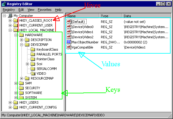
    The following image shows the tree view layout of the registry, and identifies the various items within it:

    Registry

    Querying the registry from SQL Server

    Using xp_regread / xp_instance_regread

    Let’s start off by querying some data within SQL Server. I have an instance of SQL Server named “SQL2014” (would you care to take a guess as to what version of SQL Server this is?). One of the items stored in the registry is the location of the SQL Agent working directory. These procedures can query the registry and return the specified values. For example:

    EXECUTE master.sys.xp_regread 
        'HKEY_LOCAL_MACHINE', 
        'Software\Microsoft\Microsoft SQL Server\MSSQL12.SQL2014\SQLServerAgent', 
        'WorkingDirectory';

    When I execute this statement, SQL returns the following result:

    Value            Data
    ---------------- -----------------------------------
    WorkingDirectory D:\MSSQL\MSSQL12.SQL2014\MSSQL\JOBS

    In order for you to run this, you may need to change the key as appropriate for the version and instance on your server. The result includes both the value, and the data for the specified path.

    xp_instance_regread

    In this example, I used xp_regread to read the direct registry path. If you remember from earlier, there are SQL Server instance-aware versions of each registry procedure. A comparable statement using the instance-aware procedure would be:

    EXECUTE master.sys.xp_instance_regread
        'HKEY_LOCAL_MACHINE',
        'Software\Microsoft\MSSQLSERVER\SQLServerAgent',
        'WorkingDirectory';

    This statement returns the exact same information. Let’s look at the difference between these – in the first query, the registry path is the exact registry path needed, and it includes “\Microsoft SQL Server\MSSQL12.SQL2014\”. In the latter query, this string is replaced with “\MSSQLSERVER\”. Since the latter function is instance aware, it replaces the “MSSQLSERVER” with the exact registry path necessary for this instance of SQL Server. Pretty neat, isn’t it? This allows you to have a script that will run properly regardless of the instance that it is being run on. The rest of the examples in this post will utilize the instance-aware procedures to make it easier for you to follow along and run these yourself.

    Syntax

    The syntax for these procedures is:

    EXECUTE xp_regread 
        [@rootkey=]’rootkey’,
        [@key=]’key’
        [, [@value_name=]’value_name’]
        [, [@value=]@value OUTPUT]

    The first parameter is the registry hive that you want to query, the second parameter is the key path, and the third is the value name. The third parameter is optional – if it is provided, then the procedure will return the data from the specified value item; if it is not provided, then the procedure only returns whether the specified key exists. There is also an optional fourth parameter, which is an output parameter, and the data output will go into that. The parameters are positional, and while you can specify a name for the parameter, any name will work. Since the parameters are positional, my recommendation is to not use the parameter names. The following example utilizes the optional fourth parameter, and it will return just the specified path into the variable:

    DECLARE @SQLAgentDirectory VARCHAR(255);
    EXECUTE master.sys.xp_instance_regread
        'HKEY_LOCAL_MACHINE',
        'Software\Microsoft\MSSQLSERVER\SQLServerAgent',
        'WorkingDirectory',
        @SQLAgentDirectory OUTPUT;
    SELECT @SQLAgentDirectory;

    You would think that if you specify either NULL or an empty string for the third parameter, that you could send whether the key exists to an output variable – however, I have not been able to figure out a way to accomplish this. Specifying either of these values results in an error when running this statement. If you know how to do this, please leave a remark so that this post can be updated with that information.

    Using xp_regenumvalues / xp_instance_regenumvalues

    These procedures will enumerate through all of the values of the specified key, returning a separate result set for each value. For instance, the following statement will return all of the values in the above SQLServerAgent key:

    EXECUTE master.sys.xp_instance_regenumvalues
        'HKEY_LOCAL_MACHINE',
        'Software\Microsoft\MSSQLSERVER\SQLServerAgent';

    Having all of these result sets makes it difficult to work with this procedure. Thankfully, you can put these all into one result set – just create a temporary table (or table variable) to hold the output, and then use INSERT / EXECUTE to fill it, like the following example does:

    DECLARE @Registry TABLE (Value VARCHAR(255), Data VARCHAR(255));
    INSERT INTO @Registry
    EXECUTE master.sys.xp_instance_regenumvalues
        'HKEY_LOCAL_MACHINE',
        'Software\Microsoft\MSSQLSERVER\SQLServerAgent';
    SELECT * FROM @Registry;

    Now that all of the results are in one result set, you can work with it a bit easier.

    Syntax

    The syntax for these procedures is:

    EXECUTE xp_regenumvalues 
        [@rootkey=]’rootkey’,
        [@key=]’key’

    Using xp_regenumkeys / xp_instance_regenumkeys

    These procedures will enumerate through all of the keys in a specified path, and return all of the keys in that path. Unlike xp_instance_regenumvalues, all of the keys are returned in one result set, though you will probably want to use INSERT / EXECUTE to put this into temporary storage so that you can work with it. An example of using these procedures is:

    EXECUTE master.sys.xp_instance_regenumkeys
        'HKEY_LOCAL_MACHINE',
        'Software\Microsoft\MSSQLSERVER';

    The syntax for these procedures is:

    EXECUTE xp_regenumkeys 
        [@rootkey=]’rootkey’,
        [@key=]’key’

    Modifying the registry from within SQL Server

    Up to this point, we have focused on retrieving data from the registry. What if you want to modify the registry? Read on… be forewarned that the following procedures are modifying the registry, which means that they can also damage the registry, possibly rendering the server unusable. Use at your own risk!

    xp_regwrite / xp_instance_regwrite

    These procedures are used to create keys and write data into the registry. You can create up to 32 sub-keys at a time. In the following example, a new key “MyNewKey” will be added to the SQLServerAgent key, and the value “MyNewValue” will be added to this new key with the data “Now you see me!”. It will then read this value from the registry.

    EXECUTE master.sys.xp_instance_regwrite
        'HKEY_LOCAL_MACHINE',
        'Software\Microsoft\MSSQLSERVER\SQLServerAgent\MyNewKey',
        'MyNewValue',
        'REG_SZ',
        'Now you see me!';
    EXECUTE master.sys.xp_instance_regread
        'HKEY_LOCAL_MACHINE',
        'Software\Microsoft\MSSQLSERVER\SQLServerAgent\MyNewKey',
        'MyNewValue';

    Syntax

    The syntax for these procedures is:

    EXECUTE xp_regwrite 
        [@rootkey=]’rootkey’,
        [@key=]’key’,
        [@value_name=]’value_name’,
        [@type=]’type’,
        [@value=]’value’

    xp_regdeletevalue / xp_instance_regdeletevalue

    These procedures are used to delete a specified value from the registry. In this example, the “MyNewValue” value will be deleted. The example first enumerates through all of the values in this key (just the one), deletes the value, enumerates through them again (since there are no values, there will be no result set), and then finally shows that the key is still present.

    EXECUTE master.sys.xp_instance_regenumvalues
        'HKEY_LOCAL_MACHINE',
        'Software\Microsoft\MSSQLSERVER\SQLServerAgent\MyNewKey';
    EXECUTE master.sys.xp_instance_regdeletevalue
        'HKEY_LOCAL_MACHINE',
        'Software\Microsoft\MSSQLSERVER\SQLServerAgent\MyNewKey',
        'MyNewValue';
    EXECUTE master.sys.xp_instance_regenumvalues
        'HKEY_LOCAL_MACHINE',
        'Software\Microsoft\MSSQLSERVER\SQLServerAgent\MyNewKey';
    EXECUTE master.sys.xp_instance_regread
        'HKEY_LOCAL_MACHINE',
        'Software\Microsoft\MSSQLSERVER\SQLServerAgent\MyNewKey';

    Syntax

    The syntax for these procedures is:

    EXECUTE xp_regdeletevalue 
        [@rootkey=]’rootkey’,
        [@key=]’key’,
        [@value_name=]’value_name’

    xp_regdeletekey / xp_instance_regdeletekey

    These procedures are used to delete an entire key from the registry. In this example, the script will first add another new key under “MyNewKey”, and a value in that new key. The script then deletes both the “AnotherNewKey” (which deletes the value just added also) and “MyNewKey” keys and finally shows that both keys have been deleted. Note that in order to delete a key, it cannot have any sub-keys, which is why the script deletes “AnotherNewKey” first (try running the script first by commenting out the first xp_instance_regdeletekey to see that it must be empty).

    EXECUTE master.sys.xp_instance_regwrite
        'HKEY_LOCAL_MACHINE',
        'Software\Microsoft\MSSQLSERVER\SQLServerAgent\MyNewKey\AnotherNewKey',
        'MyNewValue',
        'REG_SZ',
        'Another new value!';
    EXECUTE master.sys.xp_instance_regread
        'HKEY_LOCAL_MACHINE',
        'Software\Microsoft\MSSQLSERVER\SQLServerAgent\MyNewKey\AnotherNewKey';
    EXECUTE master.sys.xp_instance_regdeletekey
        'HKEY_LOCAL_MACHINE',
        'Software\Microsoft\MSSQLSERVER\SQLServerAgent\MyNewKey\AnotherNewKey';
    EXECUTE master.sys.xp_instance_regdeletekey
        'HKEY_LOCAL_MACHINE',
        'Software\Microsoft\MSSQLSERVER\SQLServerAgent\MyNewKey';
    EXECUTE master.sys.xp_instance_regread
        'HKEY_LOCAL_MACHINE',
        'Software\Microsoft\MSSQLSERVER\SQLServerAgent\MyNewKey\AnotherNewKey';
    EXECUTE master.sys.xp_instance_regread
        'HKEY_LOCAL_MACHINE',
        'Software\Microsoft\MSSQLSERVER\SQLServerAgent\MyNewKey';

    Syntax

    The syntax for these procedures is:

    EXECUTE xp_regdeletekey 
        [@rootkey=]’rootkey’,
        [@key=]’key’

    xp_regaddmultistring / xp_instance_regaddmultistring

    These procedures are used to add a string to a multi-string entry in the registry, or to create a multi-string registry entry. In this example, I’ll call the procedure twice. The first time will create the entry with one string in it, and the second time will add a second string to it. Then the example will show the results of this value.

    EXECUTE master.sys.xp_instance_regaddmultistring
        'HKEY_LOCAL_MACHINE',
        'Software\Microsoft\MSSQLSERVER\SQLServerAgent\MyNewKey',
        'MyNewValue',
        'A multi-string value!';
    EXECUTE master.sys.xp_instance_regaddmultistring
        'HKEY_LOCAL_MACHINE',
        'Software\Microsoft\MSSQLSERVER\SQLServerAgent\MyNewKey',
        'MyNewValue',
        'Yet Another new string added to this multi-string value!';
    EXECUTE master.sys.xp_instance_regread
        'HKEY_LOCAL_MACHINE',
        'Software\Microsoft\MSSQLSERVER\SQLServerAgent\MyNewKey',
        'MyNewValue'

    Did you notice that the regread procedure got a little confused here? It has two value columns (which is the name of the value), but the second one has the data for the first one. Then the data column is null. If a third string is added, it still returns just these three columns. To see that we actually added these strings, we’ll have to use regedit.exe:

    -- add a third string
    EXECUTE master.sys.xp_instance_regaddmultistring
        'HKEY_LOCAL_MACHINE',
        'Software\Microsoft\MSSQLSERVER\SQLServerAgent\MyNewKey',
        'MyNewValue',
        'How about a third string?';
    -- only shows the first string
    EXECUTE master.sys.xp_instance_regread
        'HKEY_LOCAL_MACHINE',
        'Software\Microsoft\MSSQLSERVER\SQLServerAgent\MyNewKey',
        'MyNewValue'

    Registry2

    Syntax

    The syntax for these procedures is:

    EXECUTE xp_regaddmultistring 
        [@rootkey=]’rootkey’,
        [@key=]’key’,
        [@value_name=]’value_name’,
        [@value=]’value’

    xp_regremovemultistring / xp_instance_regremovemultistring

    These procedures are used to remove a string from a multi-string entry. This example will remove the middle string.

    EXECUTE master.sys.xp_instance_regremovemultistring
        'HKEY_LOCAL_MACHINE',
        'Software\Microsoft\MSSQLSERVER\SQLServerAgent\MyNewKey',
        'MyNewValue',
        'Yet Another new string added to this multi-string value!';

    Examining the string now in regedit.exe, it can be seen that it removed all of the strings starting with the specified string… in other words, it removed the second and third strings. If we add the strings back in, and then remove the third string, we can see that it also removes the second and third string. In testing with a fourth string, it appears that if you are deleting a string that is not the first string, then all of the remainder of the strings after the first string are removed. Deleting the first string deletes all of the strings. Well, these are undocumented procedures, so it’s not likely that this bug will ever be fixed.

    Syntax

    The syntax for these procedures is:

    EXECUTE xp_regremovemultistring 
        [@rootkey=]’rootkey’,
        [@key=]’key’,
        [@value_name=]’value_name’,
        [@value=]’value’

    And finally, let’s ensure that things are cleaned up:

    EXECUTE master.sys.xp_instance_regdeletekey
        'HKEY_LOCAL_MACHINE',
        'Software\Microsoft\MSSQLSERVER\SQLServerAgent\MyNewKey';

    Conclusion

    With the exception of removing and reading the multi-string values, these extended stored procedures all work pretty well. We’ve been able to read registry values, and to enumerate through a list of keys and values. Keys and values can be created and deleted.

    If you try to use the procedures in sections outside of SQL Server keys, you may run into registry security problems where the SQL Server service account doesn’t have permissions to accomplish the task. On the internet, you will find articles telling you to add the service account to the local administrators group (and to restart the service). This is a VERY BAD IDEA – by doing this, the server can be completely compromised – you will be allowed to do anything that you desire on the server. Instead, use regedt32.exe, which will allow you to modify the permissions on the key that where you are having access issues.

    I close by repeating my warning from above – be very careful when modifying the registry. It is possible to corrupt the registry to the point where the server will no longer function. To recover, an operating system reinstall will be necessary.

    As a footnote on working with the instance-aware installation. I recall seeing on the internet other keywords that could be substituted instead of MSSQLSERVER. One of them is SQLServerAgent. However, I can’t find any others right now. If you happen to know of other keywords that work, please reply to this post so that it can be added to this post.

    This post is re-published from my original post on SQL Solutions Group.

    The post Working with the registry from within SQL Server appeared first on Wayne Sheffield.

    15 Nov 02:39

    Now available in India: Azure Database for MySQL and Azure Database for PostgreSQL

    by SQL Server Team

    We recently announced public preview availability of Azure Database for PostgreSQL and MySQL in West and Central India. PostgreSQL and MySQL are ubiquitous names in the world of open source relational databases, as these database engines have been widely embraced by developers in recent years. Microsoft’s Azure cloud is a first-class platform for open source technology that allows you to bring the tools you love, along with the skills you already have, and deploy any application. The availability of Azure Database for MySQL and PostgreSQL services in India provides app developers the ability to choose from a wider number of geographies and deploy their favorite database on Azure — without the complexity of managing and administering the databases.

    Learn more about the new availability of Azure Database for MySQL and Azure Database for PostgreSQL in our recent post on the Azure blog.

    You can create an Azure Database for MySQL by following the steps mentioned in MySQL documentation, and you can create an Azure Database for PostgreSQL by following the steps outlined in PostgreSQL documentation. As you can see from the screenshots below, the “Location” drop-down now allows you to select India as a region!

    15 Nov 02:38

    Multi-Statement TVFs in Dynamics CRM

    by Guest Posts

    Guest Author : Andy Mallon (@AMtwo)

    If you're familiar with supporting the database behind Microsoft Dynamics CRM, you probably know that it's not the fastest-performing database. Honestly, that shouldn't be a surprise–it's not designed to be a screaming-fast database. It's designed to be a flexible database. Most Customer Relationship Management (CRM) systems are designed to be flexible so that they can meet the needs of many businesses in many industries with vastly different business requirements. They put those requirements ahead of database performance. That's probably smart business, but I'm not a business person–I'm a database person. My experience with Dynamics CRM is when people come to me and say

    Andy, the database is slow

    One recent occurrence was with a report failing due to a 5-minute query timeout. With the proper indexes, we should be able to get a few hundred rows really fast. I got my hands on the query and some example parameters, dropped it into Plan Explorer, and ran it a few times in our Test environment (I'm doing all this in Test–that's going to be important later). I wanted to make sure I was running it with a warm cache, so that I could use "the best of the worst" for my benchmark. The query was a big nasty SELECT with a CTE, and a bunch of joins. Unfortunately, I can't provide the exact query, since it had some customer-specific business logic (Sorry!).

    7 minutes, 37 seconds is as good as it gets.7 minutes, 37 seconds is as good as it gets.

    Right off the bat, there's a lot of bad going on here. 1.5 million reads is a heck of a lot of I/O. 457 seconds to return 200 rows is slow. The Cardinality Estimator expected 2 rows, instead of 200. And there were a lot of writes–since this query is only a SELECT statement, this means we must be spilling to TempDb. Maybe I'll get lucky, and be able to create an index to eliminate a table scan and speed this thing up. What's the plan look like?

    Looks like an apatosaurus, or maybe a giraffe.Looks like an apatosaurus, or maybe a giraffe.

    There will be no quick hits

    Let me pause for a moment to explain something about Dynamics CRM. It uses views. It uses nested views. It uses nested views to enforce row-level security. In Dynamics parlance, these row-level-security-enforcing nested views are called "filtered views." Every query from the application goes through these filtered views. The only "supported" way to perform data access is to use these filtered views.

    Recall I said this query was referencing a bunch of tables? Well, it's referencing a bunch of filtered views. So the complicated query I was handed is actually several layers more complicated. At this point, I got a fresh cup of coffee, and switched to a bigger monitor.

    A great way to solve problems is to start at the start. I zoomed in on the SELECT operator, and followed the arrows to see what was going on:

    Zooming InEven on my 34" ultra-wide monitor, I had to fiddle with the display settings for the plan to see this much. Plan Explorer can rotate plans 90 degrees to make "tall" plans fit on a wide monitor.

    Look at all those table-valued function calls! Followed immediately by a really expensive hash match. My Spidey Sense started to tingle. What is fn_GetMaxPrivilegeDepthMask, and why is it being called 30 times? I bet this is a problem. When you see "Table-valued function" as an operator in a plan, that actually means it's a multi-statement table-valued function. If it were an inline table-valued function, it would get incorporated into the larger plan, and not be a black box. Multi-statement table-valued functions are evil. Don't use them. The Cardinality Estimator isn't able to make accurate estimates. The Query Optimizer isn't able to optimize them in the context of the larger query. From a performance perspective, they don't scale.

    Even though this TVF is an out-of-the-box piece of code from Dynamics CRM, my Spidey Sense tells me that it's the problem. Forget this big nasty query with a big scary plan. Lets step into that function and see what's going on:

    create function [dbo].[fn_GetMaxPrivilegeDepthMask](@ObjectTypeCode int) 
    returns @d table(PrivilegeDepthMask int)
    -- It is by design that we return a table with only one row and column
    as
    begin
    	declare @UserId uniqueidentifier
    	select @UserId = dbo.fn_FindUserGuid()
     
    	declare @t table(depth int)
     
    	-- from user roles
    	insert into @t(depth)	
    	select
    	--privilege depth mask = 1(basic) 2(local) 4(deep) and 8(global) 
    	-- 16(inherited read) 32(inherited local) 64(inherited deep) and 128(inherited global)
    	-- do an AND with 0x0F ( =15) to get basic/local/deep/global
    		max(rp.PrivilegeDepthMask % 0x0F)
    	   as PrivilegeDepthMask
    	from 
    		PrivilegeBase priv
    		join RolePrivileges rp on (rp.PrivilegeId = priv.PrivilegeId)
    		join Role r on (rp.RoleId = r.ParentRootRoleId)
    		join SystemUserRoles ur on (r.RoleId = ur.RoleId and ur.SystemUserId = @UserId)
    		join PrivilegeObjectTypeCodes potc on (potc.PrivilegeId = priv.PrivilegeId)
    	where 
    		potc.ObjectTypeCode = @ObjectTypeCode and 
    		priv.AccessRight & 0x01 = 1
     
    	-- from user's teams roles
    	insert into @t(depth)	
    	select
    	--privilege depth mask = 1(basic) 2(local) 4(deep) and 8(global) 
    	-- 16(inherited read) 32(inherited local) 64(inherited deep) and 128(inherited global)
    	-- do an AND with 0x0F ( =15) to get basic/local/deep/global
    		max(rp.PrivilegeDepthMask % 0x0F)
    	   as PrivilegeDepthMask
    	from 
    		PrivilegeBase priv
            join RolePrivileges rp on (rp.PrivilegeId = priv.PrivilegeId)
            join Role r on (rp.RoleId = r.ParentRootRoleId)
            join TeamRoles tr on (r.RoleId = tr.RoleId)
            join SystemUserPrincipals sup on (sup.PrincipalId = tr.TeamId and sup.SystemUserId = @UserId)
            join PrivilegeObjectTypeCodes potc on (potc.PrivilegeId = priv.PrivilegeId)
    	where 
    		potc.ObjectTypeCode = @ObjectTypeCode and 
    		priv.AccessRight & 0x01 = 1
     
    	insert into @d select max(depth) from @t
    	return	
    end		
    GO

    This function follows a classic pattern in multi-statement TVFs:

    • Declare a variable that is used as a constant
    • Insert into a table variable
    • Return that table variable

    There's nothing fancy going on here. We could re-write these multiple statements as a single SELECT statement. If we can write it as a single SELECT statement, we can re-write this as an inline TVF.

    Let's do it

    If it isn't obvious, I'm about to re-write code provided by a software vendor. I've never met a software vendor that considers this to be "supported" behavior. If you change the out-of-the-box application code, you are on your own. Microsoft certainly considers this "unsupported" behavior for Dynamics. I'm going to do it anyway, since I'm using the test environment and I'm not playing around in production. Re-writing this function took just a couple minutes–so why not give it a try and see what happens? Here's what my version of the function looks like:

    create function [dbo].[fn_GetMaxPrivilegeDepthMask](@ObjectTypeCode int) 
    returns table
    -- It is by design that we return a table with only one row and column
    as
    RETURN
    	-- from user roles
    	select PrivilegeDepthMask = max(PrivilegeDepthMask) 
    	    from	(
    	    select
                --privilege depth mask = 1(basic) 2(local) 4(deep) and 8(global) 
    	    -- 16(inherited read) 32(inherited local) 64(inherited deep) and 128(inherited global)
    	    -- do an AND with 0x0F ( =15) to get basic/local/deep/global
    		    max(rp.PrivilegeDepthMask % 0x0F)
    	       as PrivilegeDepthMask
    	    from 
    		    PrivilegeBase priv
    		    join RolePrivileges rp on (rp.PrivilegeId = priv.PrivilegeId)
    		    join Role r on (rp.RoleId = r.ParentRootRoleId)
    		    join SystemUserRoles ur on (r.RoleId = ur.RoleId and ur.SystemUserId = dbo.fn_FindUserGuid())
    		    join PrivilegeObjectTypeCodes potc on (potc.PrivilegeId = priv.PrivilegeId)
    	    where 
    		    potc.ObjectTypeCode = @ObjectTypeCode and 
    		    priv.AccessRight & 0x01 = 1
            UNION ALL	
    	    -- from user's teams roles
    	    select
                --privilege depth mask = 1(basic) 2(local) 4(deep) and 8(global) 
    	    -- 16(inherited read) 32(inherited local) 64(inherited deep) and 128(inherited global)
    	    -- do an AND with 0x0F ( =15) to get basic/local/deep/global
    		    max(rp.PrivilegeDepthMask % 0x0F)
    	       as PrivilegeDepthMask
    	    from 
    		    PrivilegeBase priv
                join RolePrivileges rp on (rp.PrivilegeId = priv.PrivilegeId)
                join Role r on (rp.RoleId = r.ParentRootRoleId)
                join TeamRoles tr on (r.RoleId = tr.RoleId)
                join SystemUserPrincipals sup on (sup.PrincipalId = tr.TeamId and sup.SystemUserId = dbo.fn_FindUserGuid())
                join PrivilegeObjectTypeCodes potc on (potc.PrivilegeId = priv.PrivilegeId)
    	    where 
    		    potc.ObjectTypeCode = @ObjectTypeCode and 
    		    priv.AccessRight & 0x01 = 1
            )x
    GO

    I went back to my original test query, dumped the cache, and re-ran it a few times. Here's the slowest run time, when using my version of the TVF:

    That looks much better!That looks much better!

    It's still not the most efficient query in the world, but it's fast enough–I don't need to make it any faster. Except… I had to modify Microsoft's code to make it happen. That's not ideal. Let's take a look at the full plan with the new TVF:

    Goodbye apatosaurus, hello PEZ dispenser!Goodbye apatosaurus, hello PEZ dispenser!

    It's still a really gnarly plan, but if you look at the start, all those black box TVF calls are gone. The super-expensive hash match is gone. SQL Server gets right down to work without that big bottleneck of TVF calls (the work behind the TVF is now inline with the rest of the SELECT):

    Big picture impact

    Where is this TVF actually used? Nearly every single filtered view in Dynamics CRM uses this function call. There are 246 filtered views and 206 of them reference this function. It is a critical function as part of the Dynamics row-level security implementation. Virtually every single query from the application to the databases calls this function at least once–usually a few times. This is a two-sided coin: on one hand, fixing this function will likely act as a turbo boost for the entire application; on the other hand, there's no way for me to do regression tests for everything that touches this function.

    Wait a second–if this function call is so core to our performance, and so core to Dynamics CRM, then it follows that everyone who uses Dynamics is hitting this performance bottleneck. We opened a case with Microsoft, and I called a few folks to get the ticket bumped along to the engineering team responsible for this code. With a little luck, this updated version of the function will make it into the box (and the cloud) in a future release of Dynamics CRM.

    This isn't the only multi-statement TVF in Dynamics CRM–I made the same type of change to fn_UserSharedAttributesAccess for another performance issue. And there are more TVFs that I haven't touched because they haven't caused problems.

    A lesson to everyone, even if you're not using Dynamics

    Repeat after me: MULTI-STATEMENT TABLE VALUED FUNCTIONS ARE EVIL!

    Re-factor your code to avoid using multi-statement TVFs. If you are trying to tune code, and you see a multi-statement TVF, look at it critically. You can't always change the code (or it may be a violation of your support contract if you do), but if you can change the code, do it. Tell your software vendor to stop using multi-statement TVFs. Make the world a better place by eliminating some of these nasty functions from your database.

    About the Author

    Guest Author : Andy MallonAndy Mallon is a SQL Server DBA and Microsoft Data Platform MVP that has managed databases in the healthcare, finance, e-commerce, and non-profit sectors. Since 2003, Andy has been supporting high-volume, highly-available OLTP environments with demanding performance needs. Andy is the founder of BostonSQL, co-organizer of SQLSaturday Boston, and blogs at am2.co.

    The post Multi-Statement TVFs in Dynamics CRM appeared first on SQLPerformance.com.

    15 Nov 02:36

    Red Hat Works to Improve Hybrid Cloud Reliability

    by Charles Roe

    The press release claims that, “Red Hat, Inc. (NYSE: RHT), the world’s leading provider of open source solutions, today announced that it will support .NET Core 2.0, the latest version of the open source .NET Core project, on Red Hat’s portfolio of open technologies. A lightweight and modular platform for creating web applications and microservices, […]

    The post Red Hat Works to Improve Hybrid Cloud Reliability appeared first on DATAVERSITY.

    15 Nov 02:36

    Data Virtualization vs Data Warehouse

    by James Serra

    Data virtualization goes by a lot of different names: logical data warehouse, data federation, virtual database, and decentralized data warehouse.  Data virtualization allows you to integrate data from various sources, keeping the data in-place, so that you can generate reports and dashboards to create business value from the data.  It is an alternative to building a data warehouse, where you collect data from various sources and store a copy of the data in a new data store.

    The main advantage of data virtualization is speed-to-market, where we can build a solution in a fraction of the time it takes to build a data warehouse.  This is because you don’t need to design and build the data warehouse and the ETL to copy the data into it, and also don’t need to spend as much time testing.  Copying the data means more hardware costs, more software licenses, more ETL flows to build and maintain, more data inconsistencies and more data governance costs, so using data virtualization can also save you a lot of money.  Other reasons for data virtualization include rapid prototyping for batch data movement, self-service analytics via a virtual sandbox, and regulatory constraints on moving data.

    Some of the more popular data virtualization products are Cisco Data Virtualization (previously called Composite Software), Denodo Platform for Data VirtualizationInformatica Data Virtualization, Drermio, IBM Big SQL and Incorta.

    Along the same lines of data virtualization vs data warehouse is federated queries vs data lake.  Such technologies as PolyBase, Metanautix, and U-SQL in Azure Data Lake Analytics provide for federated queries.

    But there are some major drawbacks to data virtualization and federated queries, so you have to ask the following questions when you are thinking about using it:

    • Speed.  Is this something I could use for a Power BI dashboard where I wanted to slice and dice data with sub-second response times?  Or is this more for operational type reporting?
    • How much will this affect the performance of the source system?  Could a query consume all the resources of a server with a data source that I’m querying against?  Does it push down the query in the same way PolyBase does?
    • Do I need to install something on each server that contains a data source I want to use?
    • Does it use the indexes of each technology on the data store, or does it create its own indexes?
    • How is security handled for giving users access to each data source?
    • How is master data management handled (i.e. the same customer in multiple data sources but the customer name spelled differently)?
    • Where and how will the data be cleaned?
    • Will reports break if the source system is changed?

    And there are some very valid reasons why a physical data warehouse is required:

    • Many production systems don’t keep track of historical data.  This data must be stored somewhere for historical analysis of the data. The physical data warehouse is, in this case, the most obvious solution
    • Accessing production systems directly for reporting and analytics can lead to too much interference on those systems and to performance degradation.  Note that this was once the reason why physical data warehouses were developed in the first place
    • Speed: I data warehouse is optimized for read access while a source system is usually optimized for writes
    • In building a data warehouse you will be restructuring, renaming, and joining data (i.e. creating star schemas) to make it easy for users to create reports
    • A data warehouse protects users against source system upgrades

    A word about Views, such as those in SQL Server, can be thought of as a “lightweight” data virtualization solution: When users need access to operational data, views can be defined directly on the operational data store or the production databases.  But views have their own issues: operations for correcting and transforming data must be added to the view definitions, because the original operations are implemented in the physical data warehouse environment and are now bypassed.  They now have to be virtualized.

    More info:

    IT pros reveal benefits, drawbacks of data virtualization software

    Experts Reconsider the Data Warehouse

    Clearly Defining Data Virtualization, Data Federation, and Data Integration

    DATA VIRTUALIZATION

    DATA FEDERATION

    Mark Beyer, Father of the Logical Data Warehouse, Guest Post

    The Logical Data Warehouse: Smart Consolidation for Smarter Warehousing

    data federation technology (data virtualization technology or data federation services)

    Logical Data Warehousing for Big Data

    The Many Uses of Data Federation

    Data Federation

    Enterprise Data Management, Part 1

    How Data Federation Can Co-exist with an EDW

    Demystifying Data Federation for SOA

    Federation Supplements The Data Warehouse – Not Either/Or, Never Was

    Counterpoint: The Data Warehouse is Still Alive

    15 Nov 02:35

    Join me: Singapore, Melbourne and Auckland this week

    by Karen Lopez

    Related posts:

    1. I am Speaking: OEMUG – Cleveland 1 Dec 2010 On Wednesday, 1 December 2010 I’ll be speaking three times...
    2. Big Data, NoSQL and Data Modeling: Big Challenges in Data Modeling Big data and NoSQL have led to big changes In...
    3. The Key to Keys at the North Texas SQL Server User Group – 17 March I’m visiting Dallas this week to speak at the North...
    15 Nov 02:34

    Local #dax measures in #powerbi reports are not visible from #Excel

    by Marco Russo

    You can connect an Excel workbook to a Power BI model in two ways:

    In both cases, you have the ability to choose either a report or a dataset to establish the connection. However, what you really get is a connection to the underlying data model, not a connection to the report.

    Why this difference is important? The issue are local DAX measures.

    If you create a report in Power BI Desktop connecting to an existing data model (on Analysis Services or on Power BI), then you can create additional measures that are local to the report. However, these measures are not exposed to external connections, because the connection to Power BI is a connection to a data model, not to a report.

    The distinction is pretty clear if you are well aware of the difference between data model and report in Power BI. Otherwise, this could be confusing – and the user interface does not help you understanding this.

    The ability to select a data model by choosing a report seems like a way to get the semantic model from the report (including the local measures) rather than just a shortcut to pick the corresponding dataset.

    15 Nov 02:33

    New AMD Processor Families Compare Well to New Intel Processors

    by Glenn Berry

    After a very long period of near irrelevance in the desktop, high-end desktop (HEDT) and server processor market segments, AMD has released three new processor families based on their Zen architecture that are actually quite competitive with current Intel processor in these three market segments. These are the AMD Ryzen, AMD Ryzen Threadripper, and AMD EPYC 7000 families. We’ll skip the AMD Ryzen desktop processors for now and jump right into the AMD Ryzen Threadripper processors.

    AMD Ryzen Threadripper Processors

    On August 10, 2017, AMD finally released their new super high-end desktop (SHED) processor family, the AMD Ryzen Threadripper. There are two initial SKUs in the lineup, the 1950X and the 1920X. The $999.00 Threadripper 1950X has a base clock speed of 3.4GHz, with 16 physical cores plus SMT (which is AMD’s version of hyper-threading), so you get 32 logical cores total. The $799.00 Threadripper 1920X has a base clock speed of 3.5GHz with 12 physical cores plus SMT, for a total of 24 logical cores. Other SKUs with lower core counts will be added over the next few months.

    These first two models are actually available for sale, so this is not a “soft launch”. Multiple motherboards are also available to support this new processor family. Both models will have 32MB of L3 cache, and will have 64 PCIe 3.0 lanes available on the processor, with 60 of those lanes available for things like multiple discrete graphics cards, multiple M.2 PCIe 3.0 x4 NVMe storage devices and 10GbE networking. Both models will also have a boost clock speed of 4.0 GHz and an XFR boost clock speed of 4.2GHz.

    These new X399-based motherboards have eight DDR4 memory slots that support ECC RAM, so you can have 128GB of RAM with commodity 16GB DDR4 DIMMs. The processor itself will support up to 1TB of RAM when 128GB LR-DIMMs (Load Reduced DIMMs) are used, as these larger DIMMs become available and affordable.

    Another interesting fact about these processors is that they actually have two NUMA nodes at the hardware level. Hardware NUMA mode can be disabled in the BIOS (since some desktop/consumer software is not NUMA-aware). Figure 1 shows what Windows Server 2016 Task Manager looks like when it is configured to display NUMA nodes and hardware NUMA is enabled (and SMT is also disabled).

    clip_image001Figure 1: NUMA node display in Windows Server 2016 Task Manager


    Figure 2 shows what 32 logical processors look like in Windows Server 2016 Task Manager.

    Figure 2: Logical processor display in Windows Server 2016 Task Manager

    SQL Server 2016 has a new feature called automatic soft NUMA which is enabled by default when you have more than eight logical processors in a NUMA node. You can disable automatic soft NUMA with an sp_configure setting. Both of these initial Threadripper models have enough logical cores to let you experiment with hardware NUMA and with automatic soft NUMA in SQL Server 2016.

    This processor family is relevant for a Data Professional who might want to have a relatively affordable (especially compared to a competing Intel HEDT processor, which costs about twice as much) workstation to run large SQL Server workloads or multiple concurrent decent sized VMs on a desktop development and testing machine without being as quickly constrained by I/O, memory or processor core count limitations.

    The bottom line here is that you can buy/build a very powerful desktop machine for virtualization or heavy duty SQL Server development and testing usage for a lot less money than if you use an Intel Skylake-X HEDT platform.

    AMD EPYC 7000 Series Processors

    On June 20, AMD formally rolled out the EPYC series of processors for one and two-socket servers. These are based on the same Zen architecture used on the AMD Ryzen desktop and AMD Ryzen Threadripper processors. The series begins with two-socket processor models designed to offer more physical cores, memory bandwidth, and PCIe 3.0 lanes compared to the current Intel Scalable Processor family or the previous generation Intel Xeon E5-2600 v4 family processors.

    There are nine different models for two-socket servers, ranging from the eight-core EPYC 7251 to the 32-core EPYC 7601. All of these models have SMT, and Max Boost (AMD’s version of Turbo Boost). They also offer eight-channels of DDR4-2666 support (that have a total capacity of 2TB of RAM per socket) and 128 PCIe 3.0 lanes per socket.

    There are also three models specifically for one-socket servers (that have a P model number suffix), ranging from the 16-core EPYC 7351P to the 32-core EPYC 7551P. You can use a non-P SKU in a one-socket server. All of these models have all of the same specifications and support for SMT, Max Boost, memory capacity and PCIe 3.0 lane counts. Unlike Intel, AMD does not artificially cripple some SKUs for product differentiation purposes.

    Each physical processor has four Core Complexes (CCX) tied together with something AMD calls Infinity Fabric. Infinity Fabric consists of a Scalable Data Fabric (SDF) and a Scalable Control Fabric (SCF), and it is used for both intra-processor and socket-to-socket communication. Each physical processor shows up as four NUMA nodes in Windows Server 2016.

    AMD is really pushing the idea of a single-socket EPYC system as a better alternative to a two-socket Intel system for many server workloads. According to AMD, it will be much less expensive, yet will have plenty of cores, memory, and PCIe 3.0 lanes, along with no NUMA overhead. One key advantage AMD is touting is their Infinity Fabric modular interconnect technology, that works both within a single processor and between multiple processors.

    For SQL Server 2016/2017 usage, you would still want the “top of the line” SKU for a given physical core count, to get the most performance for each physical core license that you buy. Unlike Intel, AMD does not increase the base clock speed in the lower core count models. These EPYC systems have a lot of PCIe 3.0 lanes and very high memory density, so they might work really well for large SQL Server DW/Reporting workloads. For OLTP workloads, the key will be how much single-threaded performance AMD is able to get from this first-generation of EPYC, and how they compare to Intel’s new Skylake-SP processors. Figure 3 shows the fastest EPYC processor at each core count, which is what you would want for SQL Server usage.

    Picture5Figure 3: Preferred AMD EPYC 7000 Series Processors for SQL Server Usage

    These new processor families are game-changers for AMD. They finally have new processors that can compete with current Intel processors (depending on the particular benchmark) for significantly less money. Within the hardware enthusiast community, there is an incredible amount of pent-up hostility towards Intel for their monopolistic behavior and slow pace of processor product innovation over the past ten years. It will be interesting to see whether this sentiment is shared in the server community, and whether AMD will be able to capture some of the server market share.

    The post New AMD Processor Families Compare Well to New Intel Processors appeared first on SQLPerformance.com.

    15 Nov 02:32

    Data Platform versus SQL Server

    by Karen Lopez

    First, yes that’s a clickbait title. Apologies.

    But it confuses me that some folks are upset about Microsoft focusing on cloud services, multi-model databases and data analytics products at the same time they do SQL Server.

    So we are no longer SQL Server MVPs; we are Data Platform MVPs.

    It’s not confusing to me because as an architect for enterprise projects, I’ve always been focused on more than one product. More than one part of the data platform. More than one specialty.

    I’m guessing no one would care if we introduced ourselves as SQL Server MVPs. But I’m enjoying telling people the Data Platform story.

    No related posts yet.

    15 Nov 02:29

    Six reasons to consider SQL Server 2017—especially if you’re on Linux

    by SQL Server Team

    “Data is currency” is the rule of thumb in business. As with money, business data must be accessible, accurate, and usable across disparate contexts if an organization is to realize greater ROI while keeping costs under control. CIOs understand that the need to manage data—its location, composition, and utility—is as important as managing a balance sheet. For many companies, the solution is SQL Server, the industry gold standard for database management.

    But what about the many tech startups and cloud enterprises running open-source platforms? These organizations face challenges with reliably integrating, categorizing, and accessing all types of business data in an often-heterogeneous world of platforms, apps, and devices.

    The good news is SQL Server 2017 runs on Linux. Two Linux-based organizations, Convergent Computing and dv01, migrated to SQL Server 2017 for the capabilities and tools to manage and optimize their data “currency.” They share their stories in the new e-book, SQL Server 2017 on Linux: Top Six Reasons Companies Make the Move.

    In the e-book, leadership at Convergent and dv01 cover the benefits they gained with SQL on Linux, including:

    • Flexibility. Use familiar languages on the platform and cloud of your choice.
    • Performance. Take advantage of faster queries with simultaneous analytics and transaction processing.
    • Security. Protect your data at rest and in motion with centrally managed, Always Encrypted protection.
    • Cost. Expand your hardware options and achieve ROI more quickly with Linux.
    • Simplicity. Migrate without the complexity of advanced customizations or third-party solutions.
    • Everything built in. Reduce TCO with all the enterprise-level features you need.

    Download the free e-book to see how SQL Server 2017 can help your organization protect and optimize its data.

    25 Jul 07:42

    Data Quality in the Data Lake

    by Jennifer Zaino

    It’s been a few months since data migration and integration vendor Syncsort completed its acquisition of Data Quality solutions vendor Trillium Software. The combination of the two vendors is already proving a good fit, mirroring where the industry is going, according to Harald Smith, Director of Product Management at Trillium. As he explains it, Syncsort […]

    The post Data Quality in the Data Lake appeared first on DATAVERSITY.

    25 Jul 07:42

    Leadership for the DBA

    by John Magnabosco

    Recently I read a book titled “The 21 Irrefutable Laws of Leadership” by John Maxwell. In this book, Maxwell categories the qualities that creates a great leader. As I read this book I thought about the many managers and leaders that I have encountered in my life, including the ones that we all have read about in the history books or seen on the evening news. I saw how these qualities were exhibited in some leaders and how they resulted in exceptional leadership. I also saw how these qualities were disregarded which resulted in disaster.

    The reading of this book would be incomplete without a fair share of introspection. I saw qualities that come to me naturally; but could use some refinement and intentional growth. I saw qualities in which I really struggle to be average. It was a great comfort to read in the book’s introduction that even the author recognizes that he is weak in some of these qualities. It is also comforting to read that all of these qualities can be learned.

    As I concluded the reading of this book, I thought about the role of a DBA in light of these qualities. There are some DBAs, such as myself, who are in a role or position of leadership within their organization. There are other DBAs whose role is more of a solid technical one without any clear designation of leadership. One of the statements that Maxwell emphasizes in this book is that everyone has the opportunity for leadership even if their organizational position does not call for it. There is a clear difference between the mindset of leadership and positional leadership. The former can exist without the latter. The latter cannot be effective without the former.

    I would love to write about each of the 21 laws and how they relate to the DBA role; but it would be very likely that most reading this will not get past the first few before heading on to other blogs. There is only so much time in the day to read, right? So, for the benefit of brevity I will pull out two of these laws and provide some quick thoughts:

    The Law of the Lid: “Leadership Ability Determines a Person’s Level of Effectiveness”
    As a DBA you can possess all of the technical skills that can be acquired. You can take a poorly performing database and optimize the heck out of it. You can author the most effective and efficient T-SQL and speak to its minute intricacies. You can design an awesome database schema that is appropriately normalized and indexed. All of this can make you very effective technically; but if you cannot express your thoughts in a way that the non-technical managers of your organization can understand and be convinced to fund your efforts financially or resources you will not realize your full effectiveness.

    A DBA who has put as much effort into refining their leadership skills as they have their technical skills will flow into the category of being an exceptional DBA. Brad McGehee has often spoken and written about “How to become an exceptional DBA“. Many of the qualities that he speaks of are a great representation of the balance of technical skills and leadership qualities.

    The Law of Connection: “Leaders Touch a Heart Before They Ask for a Hand”
    The DBA role is often characterized as a fascist dictator who guards the database realm with a pack of rabid Doberman Pincers. He carries a big stick and uses it quickly leaving Developers cowering in the corner paralyzed. This certainly is not the picture of an exceptional DBA with leadership skills.

    An exceptional DBA with leadership skills will make the effort to understand the task that the Developer has been charged with and take the time to discuss solution options. When the DBA can elevate the skills and morale of the Developers then they are exhibiting leadership qualities. When the DBA is busy tearing down the Developers they are a destructive element. Think about how you speak of the Developers that you work with when you are conversing with other DBAs.

    Imagine the culture that I described at the beginning of this section where the DBA and Developers are infected with the “us vs. them” spirit. What will the response be when the DBA is in need of the Developer’s assistance? Would the DBA even approach them for help? How effective will the DBA be in their role?

    “Leaders define reality.” – John Maxwell
    “Be the change you want to see in the world.” – Mahatma Gandhi

    The post Leadership for the DBA appeared first on Simple Talk.

    25 Jul 07:42

    SQL Server 2016 helps with Best Practices

    by Wayne Sheffield

    In order for your SQL Server instance to run optimally, there are many SQL Server best practices that you need to follow. The SQL Health Check that you can have us perform on your instances looks at many of these. SQL Server 2016, which at the time of this writing is in a Release Candidate 0 state of readiness, has been changed to handle several of these best practices. This post will look at several of these changes.

    Some of the SQL Server Best Practices

    Instant File Initialization

    The first change appears during the installation of SQL Server 2016 itself. One of the best practice items that I look for in my Health Check is that the SQL Server Database Engine service has the “Perform Volume Maintenance Task” security privilege. SQL Server 2016 now allows the setting of this privilege right in the install screen.

    SSMS2016-PVMT

    The benefit of having this privilege set is that it allows SQL Server to utilize “Instant File Initialization” (IFI). When IFI is not set, then any growth of a database’s data file will be zero-initialized… that is, the entire growth portion of the file is overwritten with zeros (note that database log files are always zero-initialized initialized with 0xC0… this is needed for the crash recovery process). During the time that the database data file is being zero-initialized, no other activity can occur in the database. This setting not only affects growths of data files, but also affects database restores and adding new files to a filegroup. Kimberly Tripp has an excellent post that explains this in more detail, and the kind of performance impact that can be obtained by having IFI enabled.

    However, configuring the instance to utilize IFI has a potential negative security side-effect. If you have just dropped a database, and a growth occurs on another database, it could use the part of the drive that the other database was using. And although it is extremely unlikely, the pages could possibly line up. With advanced techniques, one could then read the data that was on those pages. Obviously, zero-initializing the pages would eliminate this problem. It is also obvious that there are a lot of circumstances that have to line up to allow this potential security issue…but the chance of it occurring will never be zero with IFI enabled.

    Because of the performance impact, and extremely low security risk, most SQL Server professionals recommend having this option set.

    tempdb

    Ahh, tempdb. In SQL Server, that database does so much… it’s where temporary tables and table variables are stored. It’s where row version activity is stored. It’s where running queries will spill out temporary workspace needed for the query. And on, and on, and on. On busy systems, having this database running optimally is of vital importance. And there are several best practices that need to be observed here.

    First up is the number of data files needed for tempdb. On a busy system that is creating a lot of temporary objects (specifically temporary tables and table variables), the creation of these objects creates a hot-spot in one of the database file’s internal page types that stores information about the allocation of these objects. However, each database file has these internal pages. Frequently, this contention can be greatly reduced by simply adding additional database files to this database. The specific advice for how many files to have has changed over time, and there is disagreement over the exact number of files to have. What isn’t disagreed over is that additional files are needed. And once again, during the SQL Server 2016 installation, this can be set, as seen in the following screen shot:

    SSMS2016-TempDB

    This screen shot shows several of the changes that are now available in the installation process. First off is the number of data files. Note that the installation limits the number of data files to the lower of 8 or the number of CPUs presented to SQL Server (one of the methods of determining how many files to have).

    The next settings that this screen shot shows is the new default size and autogrowth values. Technically, these changes are made to the model database. However, they apply to all new databases, including tempdb when it is created. The initial size of the data and log files is now 8 MB. The default auto-growth of data and log files is now 64MB.

    The next setting available in this screen is the directory to place the data and log files in. Specifically, you can have tempdb data files in multiple directories. During the installation, these files are created in the directories in a round-robin fashion.

    Trace Flags

    There are three specific trace flags that are commonly set in SQL Server. If trace flag (TF) 1117 is enabled, then whenever a data file grows, all of the files in that database will also grow. In SQL Server 2016, this trace flag has been replaced with the AUTOGROW_ALL_FLAGS or AUTOGROW_SINGLE_FILE option of the ALTER DATABASE command, and setting TF 1117 no longer has any effect. Since it is set as part of the ALTER DATABASE command, it can be controlled at the database level, where TF 1117 was a setting across the entire instance. Furthermore, because this setting is so valuable to have set in tempdb, by default tempdb is set with this feature enabled.

    TF 1118 controls whether an extent can have pages belonging to multiple objects (known as a mixed extent), or to a single object (known as a dedicated extent). Using mixed extents allows having small tables use the absolute minimum amount of storage space…which isn’t really that much of an issue as it was in SQL 7.0 when it was added. Using dedicated extents can also help in the contention when creating lots of objects really fast. In SQL Server 2016, this trace flag has been replaced with the SET MIXED_PAGE_ALLOCATION option of the ALTER DATABASE command (and like TF 1117, TF1118 no longer has any effect). Furthermore, in the tempdb database, this setting is also enabled by default.

    The next trace flag to talk about is TF 4199. This trace flag controls whether changes to how the query optimizer functions are used or not. In prior versions of SQL Server, the changes were not used unless this TF had been enabled. Starting in SQL Server 2016, most of these behaviors are enabled if the database is in the SQL Server 2016 compatibility level.

    Reference: SQL Server 2016: What’s New in (the) Database Engine

    This post is re-published from my original post on SQL Solutions Group.

    The post SQL Server 2016 helps with Best Practices appeared first on Wayne Sheffield.

    25 Jul 07:41

    Azure SQL Data Sync 2.0

    by James Serra

    Azure SQL Data Sync has been ignored for quite some time, but has finally gotten an update (it’s in public preview).  This release includes several major improvements to the service including new Azure portal support, PowerShell and REST API support, and enhancements to security and privacy.

    SQL Azure Data Sync is a Microsoft Windows Azure web service that provides data synchronization capabilities for SQL databases.  SQL Azure Data Sync allows data to be synchronized between on-premises SQL Server databases and Azure SQL databases; in addition, it can also keep multiple Azure SQL databases in sync (see Azure SQL Data Sync technical documentation).

    SQL Data Sync targets the reference data replication scenario.  Its key capabilities are:

    Sync between SQL Server (2005 SP2 and later) and Azure SQL databases, or between Azure SQL databases:

    • One-way and bi-directional sync
    • One-to-one and hub-spoke
    • Table filter and column filter
    • Scheduled and on-demand
    • Eventual consistency

    Active Geo-Replication, in contrast, targets the GeoDR scenario for Azure SQL Database by replicating the database to another region.  It only supports one-way replication (secondaries are read-only), replication is at database granularity, there is no database or column/row filter support, and it is only available for Premium service tier.

    Comparing Data Sync to transactional replication: if you only need to do one way replication, both solution work.  Transactional replication can provide better latency and transactional consistency.  But it requires more complex setup and maintenance.  It doesn’t require the latest SQL Server as publisher as SQL Server 2012 or later will work.  Data sync is an Azure Database feature which requires less maintenance and is easier to setup.  But it has a minimum five minute latency and a more significant performance impact to the source database (trigger based change tracking).  It is optimized for bi direction sync.

    Data Sync is now available in the new Azure portal.  If you would like to try Data Sync refer to this tutorial.  Existing users will be migrated to the new service starting June 1, 2017.  For more information on migration look at the blog post “Migrating to Azure SQL Data Sync 2.0.”

    More info:

    Azure SQL Data Sync Refresh

    Sync data across multiple cloud and on-premises databases with SQL Data Sync

    Getting Started with Azure SQL Data Sync (Preview)

    25 Jul 07:40

    How Mastery of Data Collection and Analysis Contributes to the Success of Amazon Prime Day

    by Hamaad Chippa

    Click to learn more about video blogger Hamaad Chippa. Amazon just completed its third-annual Amazon Prime Day (APD), a 30-hour online shopping extravaganza that offers deep discounts on popular items until quantities run out. What started as a celebration to commemorate Amazon’s 20th anniversary has quickly become a popular on-line shopping appointment, much like Cyber Monday. According to a […]

    The post How Mastery of Data Collection and Analysis Contributes to the Success of Amazon Prime Day appeared first on DATAVERSITY.

    25 Jul 07:40

    machineQ, Comcast’s Enterprise Internet of Things Service, Expanding to 12 Major U.S. Markets

    by A.R. Guess

    by Angela Guess According to a recent press release, “Comcast today announced plans to expand its enterprise Internet of Things (IoT) service, machineQ™, to 12 major U.S. markets. MachineQ is an IoT network service and platform that uses Low Power Wide Area Network (LPWAN technology based on the globally-adopted LoRaWAN™ protocol to build and deploy […]

    The post machineQ, Comcast’s Enterprise Internet of Things Service, Expanding to 12 Major U.S. Markets appeared first on DATAVERSITY.