mjpdejong

From 1952, DNA was sequenced, modified and extensively studied, but no technique was able to produce clear direct images of DNA. Now, researchers have developed a new technique to produce a direct image of the DNA helix and its inner structure.

Nature Methods 12, 806 (2015). doi:10.1038/nmeth.3572

Author: Tal Nawy

A new sequencing method identifies G-quadruplexes genome wide.

If you look at the alcohol percentage on beers, it doesn’t seem like they’re all that different. After all, a 5% lager is just 1% more alcohol than a supposedly lighter beer, right? While that’s true, Draft Magazine explains the science of how ABV actually works.

Read more...

So as a follow up to our recent article about the rather lax Windows 10 default privacy settings, Microsoft has decided that even if you aren’t upgrading – they want your data anyway. The most complete cloud indeed, made up of telemetry from your machines. Microsoft is back-porting the data harvesting portions of Windows 10 [...] The...

Read the full post at darknet.org.uk

Happy Birthday, Linux Project -- this week you turned 24. The Linux OS has grown up everywhere. Its code and the open source model are found worldwide. People often use linux without knowing it -- when they search on Google, buy metro tickets or surf the Web. Linux powers all of that infrastructure. Linux travels worldwide on airplanes, and it's embedded in many of the smart devices that bring ultra convenience to our homes and cars. It runs our WiFi routers and our Android phones and tablets.

Wetenschappelijke artikelen met korte titels krijgen over het algemeen meer aandacht, zo blijkt uit een nieuwe studie.  

Wetenschappers van de TU Delft zijn erin geslaagd om een soort kwantumnetwerk van deeltjes te bouwen over een afstand van 1,3 kilometer, een techniek waarmee in theorie ooit informatie kan worden 'geteleporteerd'. 

Quantifying a DNA, RNA or protein sample concentration is now as easy as a click of the pipette, a push of a button and a dab of tissue to clean up. Here’s what you need to know about a few of the strengths and limitations of your Nanodrop – before you set up.

Take a number, please…

A Nanodrop is a common lab spectrophotometer (you may already be familiar with the 1000 or 2000 model) that reads a single 2μl drop on a pedestal. Less prep and cleanup time means you’re able to measure several samples in under a minute, compared to what’s needed to read just one sample in a traditional cuvette! This is perfect for most lab applications, but if you’re quantifying more than 96 samples at a time for microarrays, genotyping or to send off to a core facility, you might want to utilize a Nanodrop 8000 that can read up to 8 samples simultaneously.

Tell me the source: DNA, RNA or Protein

The Nanodrop does an excellent job at measuring across a wide spectrum that spans UV and visible light. It can’t automatically determine for you that the sample on the pedestal is DNA, RNA or protein – you have to tell the software before beginning measurements so it can report an accurate concentration. Though if you happen upon a circumstance where you’ve measured half of your RNA samples at the default setting (DNA for us) you can start over again by rereading each sample at the correct software setting, or you can estimate your sample concentration by hand, based upon the raw absorbance data already collected using the table below for guidance. Remember to correct for your blank TE or water sample!

The concentration at an A260 value of 1.0 for
Double stranded DNA	50 μg/ml
Single stranded RNA	40 μg/ml
Single stranded DNA	33 μg/ml
Protein (measured at A280)	1 mg/ml

Please note that these are for relatively pure samples of DNA, RNA and protein at an A260/280 of about 1.8, 2.0 and 0.6, respectively. Additionally, the concentration of your sample will be reported in ng/μl.

Quick and dirty sample extractions: pump it up

Regardless of quantification method there are two important questions to ask after every nucleic acid extraction: Is there contamination in my sample tube? If there is, what kind is it?

From what may be read as a perfect DNA sample based upon the A260/280 alone, your Nanodrop may be overstating the results. This is a result common to most spectrophotometers: your equipment is doing what it was designed to do and that’s read absorbance at specific wavelengths.

But DNA is not the only item that absorbs at 260 nm. RNA does too. Phenol is close at about 270 nm and all of this combined has the potential to push your reported concentration upwards.

Become aware of contamination that you can see

Another point of interest is your A260/230 value, which like its A260/280 counterpart should land at or above 1.8 as a general rule of thumb, and above 2.0 for relatively pure DNA and RNA samples.

The Nanodrop paints a nice graphical picture to help you see just where attention may be needed

• Low A260/280, large peak at A280: protein contamination
• Large A230: phenol again, EDTA or carbohydrate contamination
• Small peaks or higher than expected absorbance along the far right side of the graph: contamination stemming from transfer of the interface during phase separation step in extraction.
• From the source, here’s what it can look like on your screen: 260/280 and 260/230 Ratios (ThermoScientific/Nanodrop).

One way to ensure a cleaner sample is to send it through to re-precipitation, followed by an ethanol wash, extended air-drying and re-suspension in a fresh volume of TE or pure water. Yes, your reported concentration may be significantly less than before, but that’s because you have successfully removed any contamination that was impacting your absorbance data for better or worse.

Look out below!

For the most part your nucleic acids extractions land within the measurable range of the Nanodrop (2ng – 15μg per μl). It’s when you start extracting from single cell or small sample sources that you need to consider alternative quantification methods. For example, fluorescent-dyes will help resolve amounts of DNA or RNA at or below 2ng/μl.

Want to learn more about DNA, RNA and your Nanodrop? Check out these other interesting resources:

• Nucleic Acid Quantitation (Wikipedia)
• Nanodrop (OpenWetWare)
• Quick reference: Determining DNA Concentration & Purity
• Spectrophotometer for nucleic acid measurements
• Assessment of Nucleic Acid Purity
• Where did my DNA go? Tips on improving DNA Clean-Up
• DNA Precipitation: Ethanol vs. Isopropanol
• Ethanol Precipitation of DNA and RNA: How it works

Ten years ago this month, I attended the Catalyst Workshop at the American Film Institute. The week-long program taught screenwriting to a dozen scientists, with the hope that we’d somehow help Hollywood get the science right.

But what we learned during that fabulous week, dissecting films such as “The Day After Tomorrow,”  meeting top studio people and even pitching ideas, is that the science just doesn’t matter. Although I agree that story and characters are paramount, getting the science right doesn’t take much effort, and can not only improve plausibility, but also accurately portray scientists. Geneticists in particular seem especially vulnerable to villianizing.

A TIRED PLOT
My latest target for tarnishing the image of geneticists is “Between,” a six-episode Netflix offering from Canada. (Yes, I know Halle Berry’s hybrid son on Extant has something to do with a virus, but I gave up two episodes ago.)

“Between” is an amalgam of familiar themes. It’s Logan’s Run, Under The Dome, and Lord of the Flies, with a small town setting like that of Wayward Pines, which I blogged about recently. And like those shows, the focus is on the characters and their relationships, with the predicament a backdrop that fuels the interactions.

So now we have Between. In the town of Pretty Lake, over the course of a few days, everyone aged 22 and older suddenly gasps, bleeds from the nose, and dies. The government quarantines the town and the young folk pile up the bodies of their elders and have a huge bonfire. Early in episode one, a main character, a geeky young man named, of course, Adam, mentions his father, a mysteriously missing geneticist. This is repeated throughout the early episodes. Foreshadow the mad scientist.

A nice touch is the accurate depiction of a major character who has Down syndrome. But one scene dangerously got insulin shock ass backwards. A boy with type 1 diabetes collapses from days without insulin and everyone yells “He’s in insulin shock! Give him candy!” Without insulin, how would his cells take up the glucose? Who vetted that script?

BLAME THE VIRUS
Soon, the people in Pretty Lake and the talking heads on their screens deem the culprit a virus. My husband Larry (a chemist) and I hung on through all six episodes to learn exactly how a virus could tell that a person has reached age 22.

We learn in the final episode, when the crazy nameless geneticist shows up via a tunnel that perhaps comes from Wayward Pines, that he engineered the virus. He cleverly included a bit of his own DNA so that he and his son would be immune. Note to the show’s writers: a parent and a child are not genetically identical. Nor do they have the same exposures guiding development of their immune systems.

The evil geneticist was working alone on the virus, because the government sends in unwitting workers wielding needles to “vaccinate” the town’s young survivors, supposedly so the quarantine can be lifted. But no. The shots will kill the young people to protect the rest of the world, as the clueless shotgivers over age 21 become victims, bleeding and dropping.

Larry and I were sorely disappointed with the ending, which did nothing to satisfy the craving of the scientifically-minded to understand how things work.

The geneticist explains how the virus kills people over 21 with a lot of posturing, emitting a barrage of inappropriate technical terms, concluding inexplicably with something about the ozone layer. It all speeds by too fast to process, but the spouting renegade geneticist seems to have invented the virus to fight overpopulation. I think. The focus is much more on teen angst involving a pregnancy and jealousy than how a virus can tell how old someone is.

When Adam parrots his dad’s message to the others, that the killer virus homes in on “the biological clock,” everyone nods with comprehension. But that term refers to circadian and other biorhythms, not a FitBit like contraption embedded in our spleens that flashes our exact ages. Basic Bio 101 writers! But it’s easy to see how that sort of error might have come up: oversimplification in a news release, which means oversimplification in the articles that spawn from it. The news release headline “Leicester scientists to unlock the secrets of the biological clock” actually refers to telomeres, the tips of chromosomes that whittle down with increasing age. Aha!

TELOMERES ANYONE?
The only reason that I watched “Between” to begin with was in anticipation of using telomeres in an apocalypse story. Shrinking chromosome tips are like cellular tree rings in reverse, disappearing rather than accruing with the passage of time. With repeats of TTAGGG lopped off one by one from chromosome ends as time goes on, marking the number of cell divisions, telomeres are more quantitative than gray hairs, achy joints, and wrinkles.

In telomeres, Nature provided the perfect plot point, if only the show’s writers had looked.

The telomere clock dates back to the famous “Hayflick Limit” of 40 to 60 mitoses for cells in culture. In the 1950s, Leonard Hayflick, PhD, was a young researcher at the Wistar Institute in Philadelphia. He wanted to see what the fluid around cancer cells would do to normal cells from human embryos and fetuses. At that time all cells were thought to be immortal, dividing unceasingly. “Today if I did that using federal research dollars to grow tissue from human embryos or fetuses, I would go to jail,” he told me a few years ago for my essay collection.

Hayflick had wanted to run replicates of his experiment simultaneously, but the supply of material was erratic. “In my incubator at any given time, I’d have 12 to 20 cultures going, each marked with a different start date.”

He soon discovered something strange. “Despite the fact that I used the same technician, the same glassware, and the same media, the cells in culture the longest stopped dividing, while the young cultures luxuriated. That shouldn’t happen. It intrigued me, so I began to look at what was going on.”

Hayflick’s fetal cells died after being moved a certain number of times, each move triggering cell division. He and colleague Paul Moorhead repeated their astonishing experiments over and over, with the same results – cells obeyed some sort of internal clock that marks the number of cell divisions. Freeze cells at division 20, and when thawed, they’d pick up where they left off, dividing 20 to 40 more times.

But it’s hard to change dogma and get published. And so Hayflick and Moorhead “sent the luxuriating cultures – the young ones – to the grey eminences of the field. We would tell them, ‘by May 20th to 30th, the cells are going to die.’ When the phone started ringing between May 20th and 30th, we decided to publish. If our work went up in flames, we’d be in the company of the grey eminences,” Hayflick told me. After a stinging rejection from one journal, the findings were published in Experimental Cell Research in 1961.

Discovery of the Hayflick limit founded what we now call telomere biology. Many others, including Elizabeth Blackburn, Carol Greider, and Jack Szostack, who shared the Nobel Prize for Physiology or Medicine in 2009, discovered the DNA sequence of human telomeres and how they function as fuses, marking biological time. DNA polymerase cannot replicate DNA at the end of a strand, unless an enzyme called telomerase tacks on more repeats – as happens in cancer cells. So Pretty Lake might have had a few cancer patients hanging around with the quarreling teens and kids. Their chromosome tips would appear young.

MECHANISM?

Larry and I eagerly awaited a character turning 22 to find out how the virus tracks time. Indeed, a pretty and popular teacher celebrates her 22nd birthday midway through episode 4, and sure enough, within minutes, spews nasal blood and expires. How could that have happened? After all, telomere shrinkage is not a discrete and uniform phenomenon. All 21-year-olds don’t have x number of TTAGGGs and a 22-year-old x-1.

I’m imagining deploying a virus that targets the telomeres using a form of genome editing (CRISPR/cas-9, TALENs, or zinc finger nucleases) and only integrating into a host chromosome if the number of repeats is below a certain threshhold. Then, the virus induces hemorrhage, perhaps by turning off transcription of various clotting factors. (Readers please elaborate or pose alternate hypotheses.)

Reviewers trashed Between for a lot of reasons – too derivative, “ho-hum,” a “familiar ensemble soap opera with conspiracy-theory embroidery,” and Hollywood Reporter’s “It’s the end of the world as they know it, and viewers won’t care.” None that I could find mentioned the spotty science.

I’m disturbed about the missed opportunity to imagine how a virus could take out an entire huge age cohort of humanity. But I’m much more disturbed about the tired stereotype of the mad scientist, especially the ego-driven geneticist who tailors a mysterious and dangerous virus to control human population growth. It’s not only absurd, but in this age of Ebola epidemics, and fear of vaccines and genetic modification, the ideas behind Between and the events at Pretty Lake are downright dangerous.

In deze editie pakken we het iets anders dan gebruikelijk aan. De eenvoudige, budgetvriendelijke systemen hebben we niet in een grote atx-behuizing ondergebracht, maar we houden het klein en compact.

Genomics, transcriptomics, proteomics, metabolomics – words that in 2015 sound very familiar even to a freshman in any biology field. Although most have heard those words before, I keep encountering students or even post-graduates who find it difficult to explain what they are. So, to make things easier here is a peek behind the curtains of “omics technologies”.

Word origin

In order for someone to be able to explain something, he or she should know where it comes from.

As we all know, scientists keep using Latin and Greek terminology in various fields and this also applies to our predicament.

Even from ancient Greece, medical terms used the suffix –ome, which later passed to Latin as variant –oma­ (i.e. lipoma, melanoma) and when in biology the word gene emerged, researchers quickly used the word genome to easily encapsulate a field of studies in a single word.

So, from a linguistic point of view, genome came first, and genomics after. Genomics is used to emphasize the technologies which were used to study the…genome, and if you are wondering which genome, well that’s yours.

Yes! With the human genome project being all the rage in the 90s, the term genomics was used for the first time by the consortium that was assembled in 1986. More specifically, after a long day mapping part of the human genome, beer and McDonald’s was the magic combination for Tom Roderick to propose the word to his colleagues, Frank Ruddle and Victor McKusick. He proposed it only as an idea to call a potential new scientific journal of theirs, which today is well known as Genomics.

Genomics was the first “omics” terminology used, far earlier than the second in 1995, proteomics, and so on.

So there you are, now you know where “Omics” come from, but why are they so important?

The need of inventing “Omics”

The need to create these words rose from the need to study holistic (that’s right people, another Greek word) or, if you prefer, the totality of the biology of the systems (systems biology). Soon, scientists understood that studying one gene or one metabolite or one mRNA gives little knowledge. Modern technology allows scientists to study the whole transcriptome, genome or proteome of an organism giving more and more information, so now the challenge is not to generate data, but to interpret them and to relate results of different omics technologies (i.e. trancriptomics with metabolomics).

As the technology advances and new ideas come forth, new technologies and terminologies arise. Phenomics, lipidomics, catalomics, connectomics are some of them, translating to the holistic approach of studying phenotypes, lipids, enzymes and neural connections.

So, stop thinking gene by gene, enzyme by enzyme, metabolite by metabolite and broaden your horizons to apply omics technologies for a wider knowledge of systems biology. Here are some examples on how to achieve it.

Genomics

The technologies that are focused on studying the genome of an organism including genes, exons, introns, promoters, transcription factors, and many other genome-related functions.

Technologies used: Next generation sequencing (i.e. Illumina HiSeq), Sanger sequencing, de novo assembling, bioinformatics.

Transcriptomics

The technologies that are focused on studying the transcriptome of an organism.

Technologies used: Next generation sequencing (RNA sequencing), bioinformatics, microarrays, real-time PCR.

Proteomics

The technologies that are focused on studying the proteins of an organism or the proteome.

Technologies used: Enzyme-linked immunosorbent assay (ELISA), mass spectrometric immunoassay (MSIA)

Metabolomics

The technologies that are focused on studying the metabolome or the secondary metabolites of an organism, such as amino acids, sugars, phosphates, nitrogen containing compounds, polyols, etc.

Technologies used: Gas chromatography fused with mass spectrometry (GC-MS), liquid chromatography fused with mass spectrometry (LC-MS).

Lipidomics

The technologies that are focused on studying the cellular lipids of an organism or a biological system.

Technologies used: Electrospray ionization (ESI) and matrix-assisted laser desorption/ionization (MALDI).

Catalomics

The technologies that are focused on studying enzymes (catalysts) or other biocatalysts of an organism or a system.

Technologies used: “Click” reactions in chemistry.

I think you might have stopped reading by now, so these are only some examples of “Omics” technologies and ways to approach them. This is just a brief glimpse into the technology that is here to stay. Now, it is in our hands to exploit it so basic and applied research can reap the benefits.

“Before beginning a Hunt, it is wise to ask someone what you are looking for before you begin looking for it.”

Winnie the Pooh

References

1. Babiniotis G.  (2009). The history of the words.
2. Daniel C. Liebler (2002). Introduction to proteomics: tools for the new biology. Totowa, NJ: Humana Press.
3. Karunakaran A. Kalesh et. al.(2010). The use of click chemistry in the emerging field of catalomics. Org Biomol Chem.  8(8):1749-62
4. Kopka J. (2006). Current challenges and developments in GC-MS based metabolite profiling technology. J Biotechnol. Jun 25;124(1):312-22.
5. McGettigan PA. (2013). Transcriptomics in the RNA-seq era. Curr Opin Chem Biol. Feb;17(1):4-11.
6. Yadav SP. (2007). The Wholeness in Suffix -omics, -omes, and the Word Om. Journal of Biomolecular Techniques. Dec 18(5):277.
7. McCouch SR. (2001). Genomics and Synteny. Plant. Physio. Jan;125(1):152-5.
8. Wenk MR (2005). The emerging field of lipidomics. Nat Rev Drug Discov 4 (7): 594–610.

 

How scientists study the effects of marijuana on the brain is changing. Until recently marijuana research largely excluded tobacco users from its participant pool, but scientists have found reason to abandon this practice, uncovering significant differences in the brains of individuals who use both tobacco and marijuana and the brains of those who only use […]...

Zwitserse biochemici presenteerden maandag een manier om data op te slaan in dna dat in een matrix van silicium bolletjes werd ingekapseld. Het gesynthetiseerde dna vertoonde heel weinig achteruitgang in het silicium, wat het geheel geschikt maakt voor langdurige dataopslag.

Microsoft's new unified services agreement includes language that has some worrying Microsoft may scan their Windows 10 devices for pirated software and block its use.

De novo mutations — sequence variants that are present in a child but absent from both parents — are an important source of human genetic variation. I think it’s reasonable to say that most of the 3-4 million variants in any individual’s genome arose, once upon a time, as de novo mutations in his or her ancestors. […]...

Are humans changing the course of evolution in wild fish populations? A new study making media waves today provides tantalizing evidence of a mechanism by which this may happen. In our new Naturally Speaking Reports, one of our editors caught up with Institute Senior Research Fellow Shaun Killen, the author of the study, to find out more about […]...

Intel heeft zijn eerste processors met codenaam Skylake uitgebracht. We hebben deze zesde generatie Core-processors getest met de i7-6700K en een Z170-moederbord.

We give a lot of troubleshooting help on RNA and DNA extraction here at Bitesize Bio because almost everything we do in molecular biology requires DNA or RNA at the very first step.  These days, most labs use commercial DNA extraction kits, which employ spin columns, for the isolation of DNA and RNA. The spin columns contain a silica resin that selectively binds DNA and RNA, depending on the salt conditions and other factors influenced by the extraction method.

These DNA extraction kits make the whole process much easier and faster than the methods of old, when things are going well, but the downside of using a kit is that if you don’t understand what is in the black box of the kit, it makes troubleshooting much more difficult.

So in this article, I’ll explain in some detail  how RNA and DNA extraction kits work and what is going on at each step. I’ll also go over some common problems specific to using silica columns in DNA extraction that can be overcome or avoided with just a little extra understanding.

The First Step in RNA and DNA Extraction: Lysis

The lysis formulas may vary based on the whether you want to extract DNA or RNA, but the common denominator is a lysis buffer containing a high concentration of chaotropic salt. Chaotropes destabilize hydrogen bonds, van der Waals forces,  and hydrophobic interactions. Proteins are destabilized, including nucleases, and the association of nucleic acids with water is disrupted setting up the conditions for the transfer to silica.

Chaotropic salts include guanidine HCL, guanidine thiocyanate, urea, and lithium perchlorate.

Besides the chaotropes, there is usually some detergents in the lysis buffer to help with protein solubilization and lysis. There can also be enzymes used for lysis depending on the samples type. Proteinase K is one of these, and actually works very well in these denaturing buffers; the more denatured the protein, the better Proteinase K works. Lysozyme, however, does not work in the denaturing and so lysozyme treatment is usually done before adding the denaturing salts.

One comment about plasmid preps, the lysis is very different than extraction for RNA or genomic DNA extraction because the plasmid has to be separated from the genomic DNA first and if you throw in chaotropes, you’ll release everything at once and won’t be able to differentially separate the small circular DNA from the high molecular weight chromosome.  So, in plasmid preps the chaotropes are not added until after lysis and the salts are used for binding. An excellent in-depth article on alkaline lysis is here and also another article on the difference between genomic DNA and plasmid is available for further reading.

After DNA Extraction Comes Purification: Binding the DNA to the Column

The chaotropic salts are critical for lysis, but also for binding the DNA (or RNA) to the column, as we discussed. Additionally, to enhance and influence the binding of nucleic acids to silica, alcohol is also added.

Most of the time this is ethanol but sometimes it may be isopropanol. The percent ethanol and the volume has big effects. Too much and you’ll bring in a lot of degraded nucleic acids and small species that will influence UV260 readings and throw off some of your yields.  Too little, and it may become difficult to wash away all of the salt from the membrane.

The important point here is that the ethanol influences binding and the amount added is optimized for whatever kit you are using. Modifying that step can help change what you recover so if you are having problems and want to troubleshoot recovery, that can be a step to evaluate further.

Another way to diagnose problems is to save the flow-through after binding and precipitate it to see if you can find the nucleic acids you are searching for. If you used an SDS-containing detergent in lysis, try using NaCl as a precipitant to avoid contamination of the DNA or RNA with detergent.

Washing the DNA (or RNA)

Your lysate was centrifuged through the silica membrane and now your extracted DNA or RNA should be bound to the column and the impurities, protein and polysaccharides, should have passed through.  But, the membrane is still dirty with residual proteins and salt. If the sample was from plants, there will still be polysaccharides, maybe some pigments too, left on the membrane, or if the sample was blood, the membrane might be tinted brown or yellow.

The wash steps serve to remove these impurities.  There are typically two washes, although this can vary depending on the sample type. The first wash will often have a low amount of chaotropic salt to remove the protein and colored contaminants. This is always followed with an ethanol wash to remove the salts. If the prep is something that didn’t have a lot of protein to start, such as plasmid preps or PCR clean up, then only an ethanol wash is needed.

Removal of the chaotropic salts is crucial to getting high yields and purity DNA or RNA. Some kits will even wash the column with ethanol twice. If salt remains behind, the elution of nucleic acid is going to be poor, and the A230 reading will be high, resulting in low 260/230 ratios.

For Ethanol-Free DNA and RNA, You Need a Dry Spin

After the ethanol wash, most protocols have a centrifugation step to dry the column. This is to remove the ethanol and is essential for a clean eluant. When 10 mM Tris buffer or water is applied to the membrane for elution, the nucleic acids can become hydrated and will release from the membrane. If the column still has ethanol on it, then the nucleic acids cannot be fully rehydrated.

Skipping the drying step results in ethanol contamination and low yields. I do not see ethanol absorbance on the Nanodrop, so it won’t show up in your readings. The main indicators of a problem are that when you try to load the sample onto an agarose gel, the DNA will not sink. Even in the presence of loading dye.  Another indicator is that if you put the sample in the -20C, it doesn’t freeze.

RNA and DNA Extraction, the Final Frontier: Elution

The final step in the DNA extraction protocol is the release of pure DNA or RNA from the silica.

For DNA preps, 10 mM Tris at a pH between 8-9 is typically used. DNA is more stable at a slightly basic pH and will dissolve faster in a buffer. This is true even for DNA pellets. Water tends to have a low pH, as low as 4-5 and high molecular weight DNA may not completely rehydrate in the short time used for elution. Elution of DNA can be maximized by allowing the buffer to sit in the membrane for a few minutes before centrifugation.

RNA, on the other hand, is fine at a slightly acidic pH and so water is the preferred diluent. RNA dissolves readily in water.

What Other Things Can Go Wrong with RNA and DNA Extraction

Low yields: If you experience DNA / RNA yields lower than you expected for a sample, there are many factors to think about. Usually it is a lysis problem. Incomplete lysis is a major cause of low yields. It could also be caused by incorrect binding conditions.  Make sure to use fresh high quality ethanol (100% 200 proof) to dilute buffers or for adding to the binding step. Low quality ethanol or old stocks may have taken on water and not be the correct concentration. If the wash buffer is not made correctly, you may be washing off your extracted DNA or RNA.

Low Purity: If the extracted DNA is contaminated with protein (low 260/280) then maybe you started with too much sample and the protein was not completely removed or dissolved.  If the DNA has poor 260/230 ratio the issue is usually salt from the bind or the wash buffer. Make sure that the highest quality ethanol was used to prepare wash buffers and if the problem continues, give the column an additional wash.

Some samples have a lot more inhibitors compared to others. Environmental samples are especially prone to purity issues because humic substances are solubilized during extraction. Humics behave similarly to DNA and are difficult to remove from the silica column. For this type of sample, specialized techniques exist to remove the protein and humics prior to the column step.

Degradation: This is more of a concern for RNA preps and an article that gives specific advice is here.  Mainly with RNA extractions, degradation occurs from improper storage of the sample or an inefficient lysis, assuming of course that you eluted with RNase-free water. For DNA extractions, degradation is not a huge problem because for PCR, the DNA can be sheared and it works fine. But if you were hoping to not have so much sheared DNA, then you may have used too strong a lysis method.

PCR Clean-up Special Considerations: PCR cleanup obviously isn’t a DNA extraction technique per se, but it is a nice and easy techniques, because it is simply adding a high concentration of binding salts (typically between 3-5 volumes of salt per volumes of PCR reaction) and centrifugation through the column. So when PCR Clean-up kits fail, it can be particularly frustrating.  The first question I ask people is “did you check the results of the PCR on a gel?” because you cannot UV check a PCR reaction and have an accurate reading. There is way too much in a PCR reaction absorbing UV at 260: nucleotides, detergents, salts, and primers. In my experience, a failure of a PCR clean-up kit to work frequently is caused by a PCR reaction that has failed and so there was nothing to clean up. But if you know you had a strong PCR product, the best approach is to just save your flow-through fraction after binding. If the DNA doesn’t bind, that’s where it is. You can always rescue it and then clean it up again. And then call tech support and ask for a replacement kit.

Go Forth and Perform Your RNA and DNA Extractions with Confidence

As scientists, of course we want to know exactly what is going on with our experiments and be able to troubleshoot without having to call technical service first.

I hope that this article helps clarify some of the science around the silica spin filter method for RNA and DNA extractions so you can make your own diagnosis and fixes.  So, when you do call technical service, you’ll have double checked a few of the most likely causes of problems first and instead of going through a lot of rigmarole, you can get to a resolution much faster. Even if that is a free replacement DNA extraction kit!

Any questions? Any other problems with silica spin filter preps that you don’t understand? Let us know or ask a question in our “Questions” section and we’ll discuss!

Originally published on June 28, 2010. Updated and revised on July 11, 2015.

Scientists have worked for many years to refine the technique of DNA origami. His aim is to compose new sets of design rules, vastly expanding the range of nanoscale architectures generated by the method. In new research, a variety of innovative nanoforms are described, each displaying unprecedented design control.

In studying how cells recycle the building blocks of DNA, scientists have discovered a potential therapeutic strategy for cancer. They found that normal cells have highly selective mechanisms to ensure that nucleosides -- the chemical blocks used to make new strands of DNA -- don't carry extra, unwanted chemical changes. But the scientists also found that some types of cancer cells aren't so selective. These cells incorporate chemically modified nucleosides into their DNA, which is toxic to them. The findings indicate that it might be possible to use modified nucleotides for specific killing of cancer cells.

The latest Top500 list of supercomputers is out and Linux, as ever, is the top pick for the world's fastest computers.

Normal cells are unable to replicate past several rounds of proliferation (termed the Hayflick limit) as with each round of proliferation the telomeres shorten. When the telomeres reach a critically reduced length, DNA damage is triggered leading to cellular senescence.

Therefore, if you tried to culture a primary cell population it would eventually die unless the cells were manipulated in some way to circumvent the process of senescence and become immortal. Here we discuss various ways to overcome the hayflick limit and induce immortality in cultured cells.

Sources of Imortality

Spontaneously Immortalized Cells

The best example of this would be cancer cells, which may have undergone genetic changes to resist senescence and are immortal. However, many cancer cell lines may not have these changes, in fact, George Gey, the scientist who created the first immortalized and arguably the most famous cell line: HeLa cells, had to test hundreds of cancer lines before stumbling upon the highly metaplastic ovarian cells of Henrietta Lacks. Thus, other methodologies may be required to help even cancer cells become immortal.

Introduce a Viral Gene that Overrides the Cell Cycle

Many viral genes affect the cell cycle and thus can be used to overcome senescence by removing the biological brakes on proliferative control. Many of these are tumor suppressor genes, since they require suppression for tumorigenesis to occur. The most common of these is over-expression of the Large T-antigen of the simian virus (SV-40), which represses the retinoblastoma (Rb) and p53 genes, both critical controllers of the cell cycle.

One example of a cell line immortalized with SV40 is HEK293T, which are also known as 293T cells, a cell line widely used to express viral particles and for many cellular assays, since they are very easily transfected. Other viral genes include those from the human papilloma virus (HPV) such as E6 and E7, which also target Rb and p53.

Expression of Genes that Confer Immortality

The most well-known immortality gene is Telomerase (hTERT). A ribonucleoprotein, telomerase is able to extend the DNA sequence of telomeres, thus abating the senescence process and enabling the cells to undergo infinite cell divisions. Indeed, telomerase has recently been heralded as a potential mechanism to reverse aging. The issue with using telomerase to reverse ageing is that increased telomerase expression can also induce tumor growth. Indeed, many of the same genes used to create immortalized cell lines such as hTERT and SV40 induce tumor formation. Thus, it is unsurprising that hTERT is often found over-expressed in human tumors, thus imparting one of the key hallmarks of cancer: unrestrained proliferation. Exactly what we use it for when immortalizing a primary cell line!

Combining Tumor Suppressor Inactivation and Telomerase Expression

In some cell types, using only one immortalization method may yield low numbers of cells that have become immortal. Therefore, depending on your cell line, it may be beneficial to combine both suppression of a tumor suppressor (such as the cell cycle inhibitors mentioned above) and expression of hTERT to immortalize a larger number of cells. This dual method is also suggested if you wish to both immortalize and transform (i.e. make tumorigenic-like) your cell line, as evidence suggests that some cell lines do not undergo efficient transformation without some immortalization.

How to Introduce Immortality to a Primary Cell Line

Many of the above sources of immortality are based on genetic manipulation of your primary cell line. This requires the introduction of foreign DNA into your cells. As many primary cells lines are frustratingly difficult to transfect, the easiest and most effective way to introduce genetic changes into a primary cell line is through viral infection.

The most popular method is through replication-deficient lentiviruses, since they are relatively safer then adenoviruses which have the ability to re-infect cells and thus contain live virus for a much longer period of time. If you want more information on lentiviral production, check out the Bitesize Bio Webinar and the Addgene Lentiviral Resource Page. Retroviruses can also be used to transfect cells, however, they can only infect actively dividing cells, thus reducing the number of cells that may be transduced with virus.

Words of Caution: Immortality May Not be the Best Route!

By introducing genetic changes into your cells, you may be profoundly altering the phenotype of your cell line. Although this does make your cell line more useful in some ways: it may make your cells more homogeneous allowing for replication of results, you can create large stocks of cells for future use and they may be easier to experimentally, there is still many benefits to using primary cell lines.

As primary lines adapt to being culture and being immortalized, cell populations and cellular mechanisms are altered. This may confound your experiments and lead to inconclusive or erroneous results. In addition, there is much debate about how accurately immortalized cells model real tissue. For example, although controversial, it is unlikely that SV40 can infect humans, although the mechanism of action of SV40: p53 and Rb mutations can be very common mutations in human tumors. Thus, it is important to identify the best genetic manipulation to use to immortalize your cell type.

Therefore, although immortalized cells are immensely powerful in their utility for experimental research, some caveats must be accepted in their use. As with any experimental model, immortalized cells are simply a model for your intended cellular system.

Additional Reading:

Rebecca Skloot – “The Immortal Life of Henrietta Lacks”

This is a must-read for all budding and experienced biologists. A well-researched book describes the identification of HeLa cells, their scientific value as well as the ethical dilemmas they have identified and the stress placed on the Lacks family.

References:

ATCC: HEK293T cells (ATCC CRL-3216)

Garbe et al (1999) Viral oncogenes accelerate conversion to immortality of cultured conditionally immortal human mammary epithelial cells. Oncogene. 18(13): 2169

Callaway, E (2010) Nature News: Telomerase reverses ageing process.

Hanahan & Weinberg (2011) Hallmarks of Cancer: The Next Generation. Cell. 144(5): 646.

Zhu et al (1991) The ability of simian virus 40 large T antigen to immortalize primary mouse embryo fibroblasts cosegregates with its ability to bind to p53. Journal of Virology. 65(12): 6872.

Redell (1999) The role of senescence and immortalization in carcinogenesis. Carcinogenesis. 21(3): 477.

BitesizeBio Webinar: Lentiviruses 101: Plasmids and Viral Production.

Addgene Lentiviral Protocols and Resources

Nelson (2001) Debate on the Link Between SV40 and Human Cancer Continues. Journal of the National Cancer Institute. 93(17): 1284

Sherr and McCormick (2002) The RB and p53 pathways in cancer. Cancer Cell. 2(1): 103.

Sjon shared this story from CloudFlare.

---

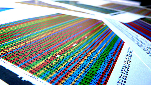
Recently I was contacted by Dr. Igor Kozin from The Institute of Cancer Research in London. He asked about the optimal way to compile CloudFlare's open source fork of zlib. It turns out that zlib is widely used to compress the SAM/BAM files that are used for DNA sequencing. And it turns out our zlib fork is the best open source solution for that file format.

CC BY-SA 2.0 image by Shaury Nash

The files used for this kind of research reach hundreds of gigabytes and every time they are compressed and decompressed with our library many important seconds are saved, bringing the cure for cancer that much closer. At least that what I am going to tell myself when I go to bed.

This made me realize that the benefits of open source go much farther than one can imagine, and you never know where a piece of code may end up. Open sourcing makes sophisticated algorithms and software accessible to individuals and organizations that would not have the resources to develop them on their own, or the money pay for a proprietary solution.

It also made me wonder exactly what we did to zlib that makes it stand out from other zlib forks.

Recap

Zlib is a compression library that supports two formats: deflate and gzip. Both formats use the same algorithm also called DEFLATE, but with different headers and checksum functions. The deflate algorithm is described here.

Both formats are supported by the absolute majority of web browsers, and we at CloudFlare compress all text content on the fly using the gzip format. Moreover DEFLATE is also used by the PNG file format, and our fork of zlib also accelerates our image optimization engine Polish. You can find the optimized fork of pngcrush here.

Given the amount of traffic we must handle, compression optimization really makes sense for us. Therefore we included several improvements over the default implementation.

First of all it is important to understand the current state of zlib. It is a very old library, one of the oldest that is still used as is to this day. It is so old it was written in K&R C. It is so old USB was not invented yet. It is so old that DOS was still a thing. It is so old (insert your favorite so old joke here). More precisely it dates back to 1995. Back to the days 16-bit computers with 64KB addressable space were still in use.

Still it represents one of the best pieces of code ever written, and even modernizing it gives only modest performance boost. Which shows the great skill of its authors and the long way compilers have come since 1995.

Below is a list of some of the improvements in our fork of zlib. This work was done by me, my colleague Shuxin Yang, and also includes improvements from other sources.

• uint64_t as the standard type - the default fork used 16-bit types.
• Using an improved hash function - we use the iSCSI CRC32 function as the hash function in our zlib. This specific function is implemented as a hardware instruction on Intel processors. It has very fast performance and better collision properties.
• Search for matches of at least 4 bytes, instead the 3 bytes the format suggests. This leads to fewer hash collisions, and less effort wasted on insignificant matches. It also improves the compression rate a little bit for the majority of cases (but not all).
• Using SIMD instructions for window rolling.
• Using the hardware carry-less multiplication instruction PLCMULQDQ for the CRC32 checksum.
• Optimized longest-match function. This is the most performance demanding function in the library. It is responsible for finding the (length, distance) matches in the current window.

In addition, we have an experimental branch that implements an improved version of the linked list used in zlib. It has much better performance for compression levels 6 to 9, while retaining the same compression ratio. You can find the experimental branch here.

Benchmarking

You can find independent benchmarks of our library here and here. In addition, I performed some in-house benchmarking, and put the results here for your convenience.

All the benchmarks were performed on an i5-4278U CPU. The compression was performed from and to a ramdisk. All libraries were compiled with gcc version 4.8.4 with the compilation flags: "-O3 -march=native".

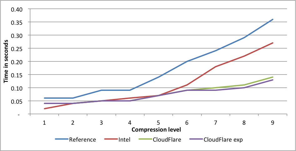
I tested the performance of the master zlib fork, optimized implementation by Intel, our own master branch, and our experimental branch.

Four data sets were used for the benchmarks. The Calgary corpus, the Canterbury corpus, the Large Canterbury corpus and the Silesia corpus.

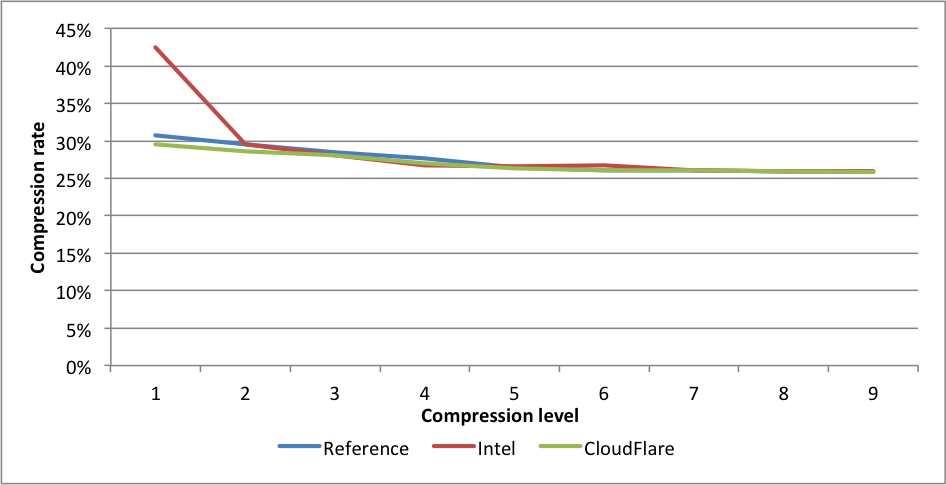
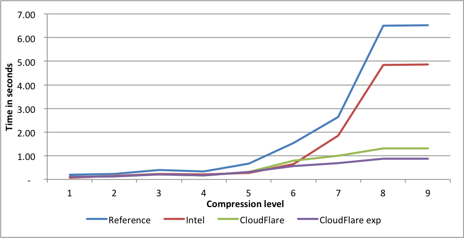
Calgary corpus

Performance:
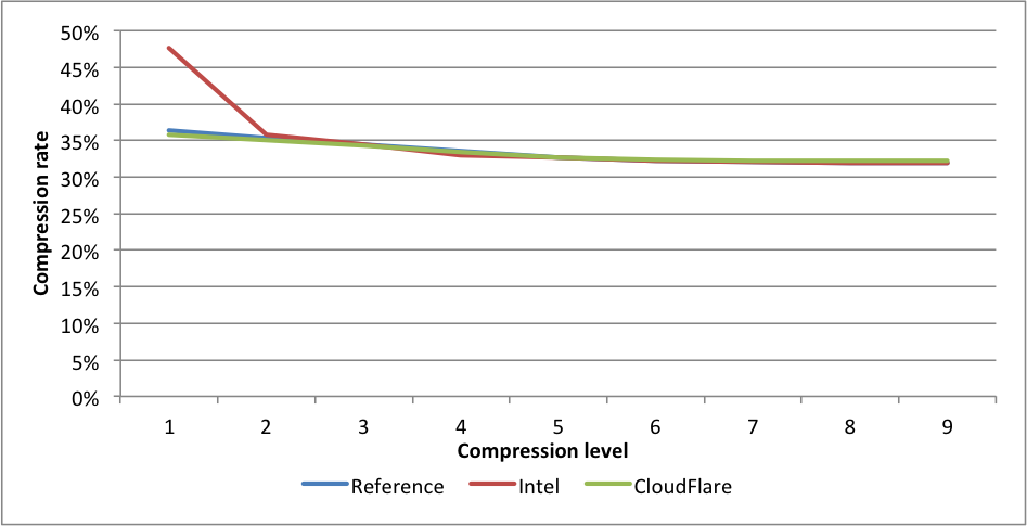
Compression rates:
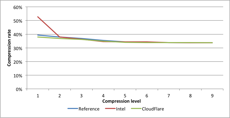For this benchmark, Intel only outperforms our implementation for level 1, but at the cost of 1.39X larger files. This difference is far greater than even the difference between levels 1 and 9, and should probably be regarded as a different compression level. CloudFlare is faster on all other levels, and outperforms significantly for levels 6 to 9. The experimental implementation is even faster for those levels.

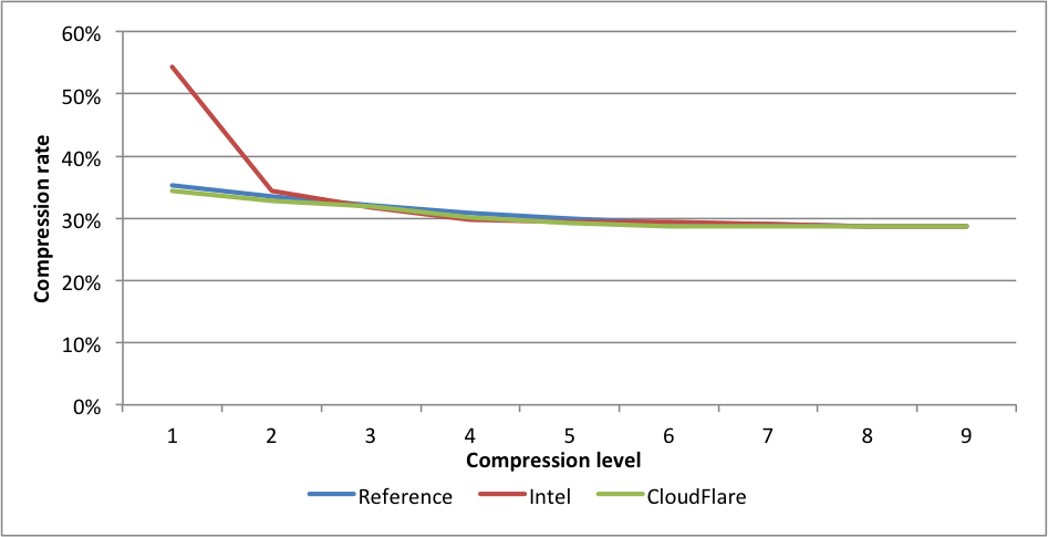
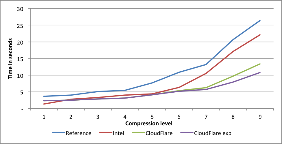
Canterbury corpus

Performance:
Compression rates:
Here we see a similar situation. Intel at level 1 gets 1.44X larger files. CloudFlare is faster for levels 2 to 9. On level 9, the experimental branch outperforms the reference implementation by 2X.

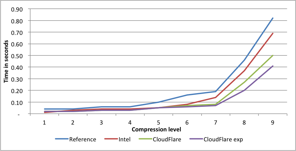
Large corpus

Performance:
Compression rates:
This time Intel is slightly faster for levels 5 and 6 than the CloudFlare implementation. The experimental CloudFlare implementation is faster still on level 6. The compression rate for Intel level 1 is 1.58 lower than CloudFlare. On level 9, the experimental fork is 7.5X(!) faster than reference.

Silesia corpus

Performance:
Compression rates:
Here again, CloudFlare is the fastest on levels 2 to 9. On level 9 the difference in speed between the experimental fork and the reference fork is 2.44X.

Conclusion

As evident from the benchmarks, the CloudFlare implementation outperforms the competition in the vast majority of settings. We put great effort in making it as fast as possible on our servers.

If you intend to use our library, you should check for yourself if it delivers the best balance of performance and compression for your dataset. As between different file format and sizes performance can vary.

And if you like open source software, don't forget to give back to the community, by contributing your own code!

An entry on ScienceDaily titled: 'Turning fake pills into real treatments' caught my eye recently and with it a link to one of the most famous placebo experiments by Ted Kaptchuk and colleagues [1] (open-access here).In the 2010 paper, Kaptchuk et al reported that even when told a placebo - a substance that has no therapeutic effect - is a placebo, when compared to a no-treatment option, participants diagnosed with irritable bowel syndrome as a group reported greater improvements in their symptoms. As per the authors' comments: "results challenge “the conventional wisdom” that placebo effects require “intentional ignorance.”"I don't mind telling you that I find this area of science to be absolutely fascinating. The placebo effect classically delivered with deception (also ideally including various information: a pill branded by a well-known pharmaceutical company, perceived as an expensive treatment accompanied by positive information from someone perceived to be a doctor and wearing a white coat) is intriguing enough but potentially even showing effects even when known to be a placebo?Granted the non-deceptive placebo response is probably not going to be generalisable across all patient groups and all conditions as per other work including Kaptchuk on the authorship list [2]. But this line of research does perhaps require quite a bit more systematic evaluation as to who might be 'best responders' and whether science can identify such people via investigations of the 'placebome' for example [3]. With the rise and rise of the science of epigenetics, one also wonders whether there may be something complementary to see there too minus any hype.Given the reliance on placebo near the top of the hierarchy of science - the placebo-controlled study - one might also reasonably ask the question as to what extent our growing knowledge of the placebo response might be affecting the quality of some of our science and what we can do about it. I'll draw your attention to a paper I have discussed before on this blog by Samokhvalov and colleagues [3] and their suggestion that: "naltrexone, upon further investigation, might be used in randomised clinical trials in addition to or as an alternative to a placebo." I'm a follower of naltrexone research on this blog (see here). Added to the possible ways and means that trial design might be adapted as per the suggestion from Sylvain Chassang and colleagues [4] and the concept of 'high' and 'low' probability of treatment being added into the statistical mix, and the Kaptchuk findings prove their worth not just when it comes to the potential effects of placebo...Music: The Doors - Riders On the Storm.----------[1] Kaptchuk TJ. et al. Placebos without deception: a randomized controlled trial in irritable bowel syndrome. PLoS One. 2010 Dec 22;5(12):e15591.[2] Kelley JM. et al. Open-label placebo for major depressive disorder: a pilot randomized controlled trial. Psychother Psychosom. 2012;81(5):312-4.[3] Samokhvalov AV. et al. Naltrexone may block euphoria-like placebo effect. BMJ Case Rep. 2013 Aug 7;2013.[4] Chassang S. et al. Accounting for Behavior in Treatment Effects: New Applications for Blind Trials. PLoS One. 2015 Jun 10;10(6):e0127227.----------Kaptchuk TJ, Friedlander E, Kelley JM, Sanchez MN, Kokkotou E, Singer JP, Kowalczykowski M, Miller FG, Kirsch I, & Lembo AJ (2010). Placebos without deception: a randomized controlled trial in irritable bowel syndrome. PloS one, 5 (12) PMID: 21203519...

Salamanders are remarkable organisms. Following the amputation or loss of complex structures such as parts of their eyes, hearts and brains, tails -including the spinal cord-, jaws and even full limbs, they are able to set up a regeneration programme which leads to the exact replacement of the missing structure, even as adults. As such, […]...

A look at living with disease close at hand, using a couple different papers. Living with Risk....

Posted by Alexander Mordvintsev, Software Engineer, Christopher Olah, Software Engineering Intern and Mike Tyka, Software Engineer

Update - 13/07/2015
Images in this blog post are licensed by Google Inc. under a Creative Commons Attribution 4.0 International License. However, images based on places by MIT Computer Science and AI Laboratory require additional permissions from MIT for use.

Artificial Neural Networks have spurred remarkable recent progress in image classification and speech recognition. But even though these are very useful tools based on well-known mathematical methods, we actually understand surprisingly little of why certain models work and others don’t. So let’s take a look at some simple techniques for peeking inside these networks.

We train an artificial neural network by showing it millions of training examples and gradually adjusting the network parameters until it gives the classifications we want. The network typically consists of 10-30 stacked layers of artificial neurons. Each image is fed into the input layer, which then talks to the next layer, until eventually the “output” layer is reached. The network’s “answer” comes from this final output layer.

One of the challenges of neural networks is understanding what exactly goes on at each layer. We know that after training, each layer progressively extracts higher and higher-level features of the image, until the final layer essentially makes a decision on what the image shows. For example, the first layer maybe looks for edges or corners. Intermediate layers interpret the basic features to look for overall shapes or components, like a door or a leaf. The final few layers assemble those into complete interpretations—these neurons activate in response to very complex things such as entire buildings or trees.

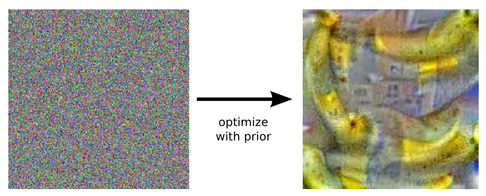
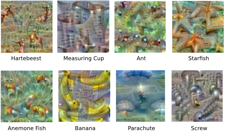
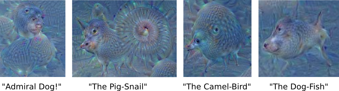
One way to visualize what goes on is to turn the network upside down and ask it to enhance an input image in such a way as to elicit a particular interpretation. Say you want to know what sort of image would result in “Banana.” Start with an image full of random noise, then gradually tweak the image towards what the neural net considers a banana (see related work in [1], [2], [3], [4]). By itself, that doesn’t work very well, but it does if we impose a prior constraint that the image should have similar statistics to natural images, such as neighboring pixels needing to be correlated.
So here’s one surprise: neural networks that were trained to discriminate between different kinds of images have quite a bit of the information needed to generate images too. Check out some more examples across different classes:
Why is this important? Well, we train networks by simply showing them many examples of what we want them to learn, hoping they extract the essence of the matter at hand (e.g., a fork needs a handle and 2-4 tines), and learn to ignore what doesn’t matter (a fork can be any shape, size, color or orientation). But how do you check that the network has correctly learned the right features? It can help to visualize the network’s representation of a fork.

Indeed, in some cases, this reveals that the neural net isn’t quite looking for the thing we thought it was. For example, here’s what one neural net we designed thought dumbbells looked like:
There are dumbbells in there alright, but it seems no picture of a dumbbell is complete without a muscular weightlifter there to lift them. In this case, the network failed to completely distill the essence of a dumbbell. Maybe it’s never been shown a dumbbell without an arm holding it. Visualization can help us correct these kinds of training mishaps.

Instead of exactly prescribing which feature we want the network to amplify, we can also let the network make that decision. In this case we simply feed the network an arbitrary image or photo and let the network analyze the picture. We then pick a layer and ask the network to enhance whatever it detected. Each layer of the network deals with features at a different level of abstraction, so the complexity of features we generate depends on which layer we choose to enhance. For example, lower layers tend to produce strokes or simple ornament-like patterns, because those layers are sensitive to basic features such as edges and their orientations.

Left: Original photo by Zachi Evenor. Right: processed by Günther Noack, Software Engineer

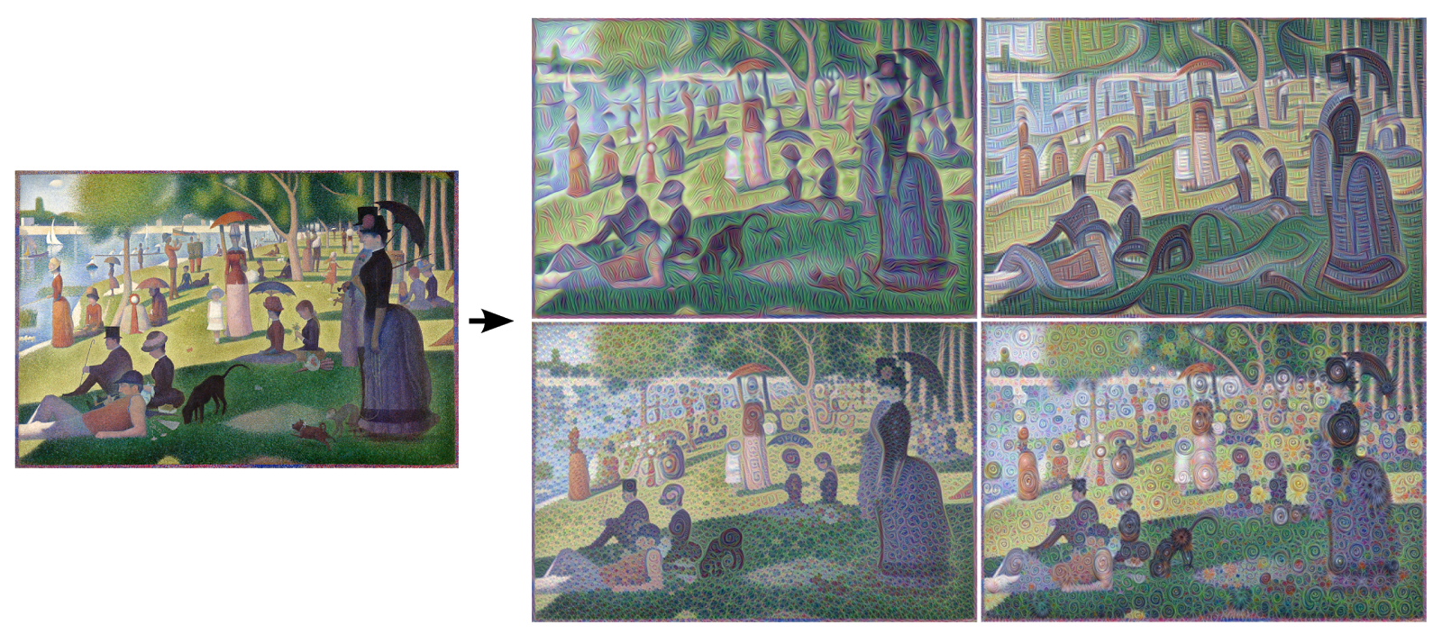Left: Original painting by Georges Seurat. Right: processed images by Matthew McNaughton, Software Engineer

If we choose higher-level layers, which identify more sophisticated features in images, complex features or even whole objects tend to emerge. Again, we just start with an existing image and give it to our neural net. We ask the network: “Whatever you see there, I want more of it!” This creates a feedback loop: if a cloud looks a little bit like a bird, the network will make it look more like a bird. This in turn will make the network recognize the bird even more strongly on the next pass and so forth, until a highly detailed bird appears, seemingly out of nowhere.
The results are intriguing—even a relatively simple neural network can be used to over-interpret an image, just like as children we enjoyed watching clouds and interpreting the random shapes. This network was trained mostly on images of animals, so naturally it tends to interpret shapes as animals. But because the data is stored at such a high abstraction, the results are an interesting remix of these learned features.
Of course, we can do more than cloud watching with this technique. We can apply it to any kind of image. The results vary quite a bit with the kind of image, because the features that are entered bias the network towards certain interpretations. For example, horizon lines tend to get filled with towers and pagodas. Rocks and trees turn into buildings. Birds and insects appear in images of leaves.

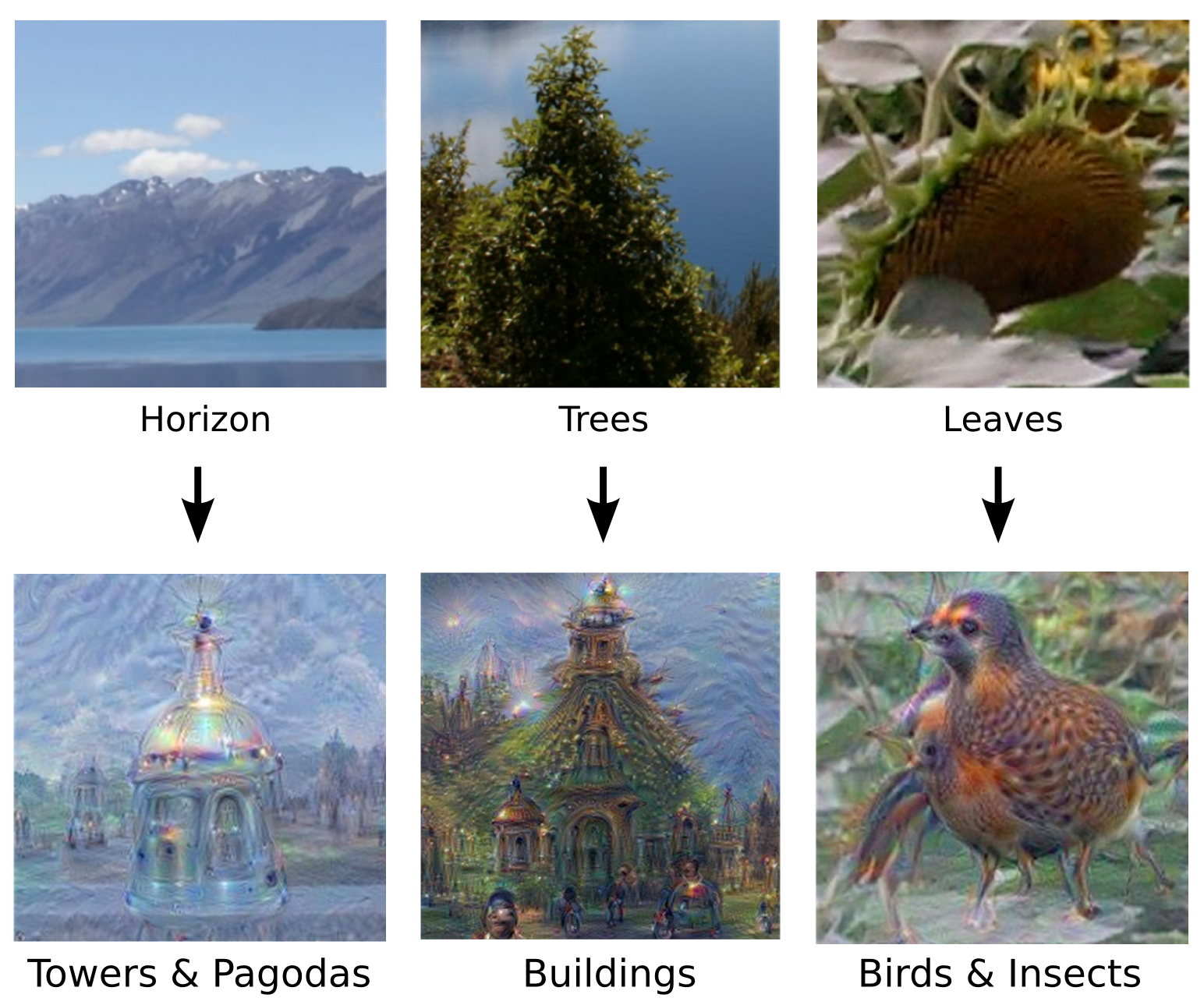The original image influences what kind of objects form in the processed image.

This technique gives us a qualitative sense of the level of abstraction that a particular layer has achieved in its understanding of images. We call this technique “Inceptionism” in reference to the neural net architecture used. See our Inceptionism gallery for more pairs of images and their processed results, plus some cool video animations.

We must go deeper: Iterations

If we apply the algorithm iteratively on its own outputs and apply some zooming after each iteration, we get an endless stream of new impressions, exploring the set of things the network knows about. We can even start this process from a random-noise image, so that the result becomes purely the result of the neural network, as seen in the following images:

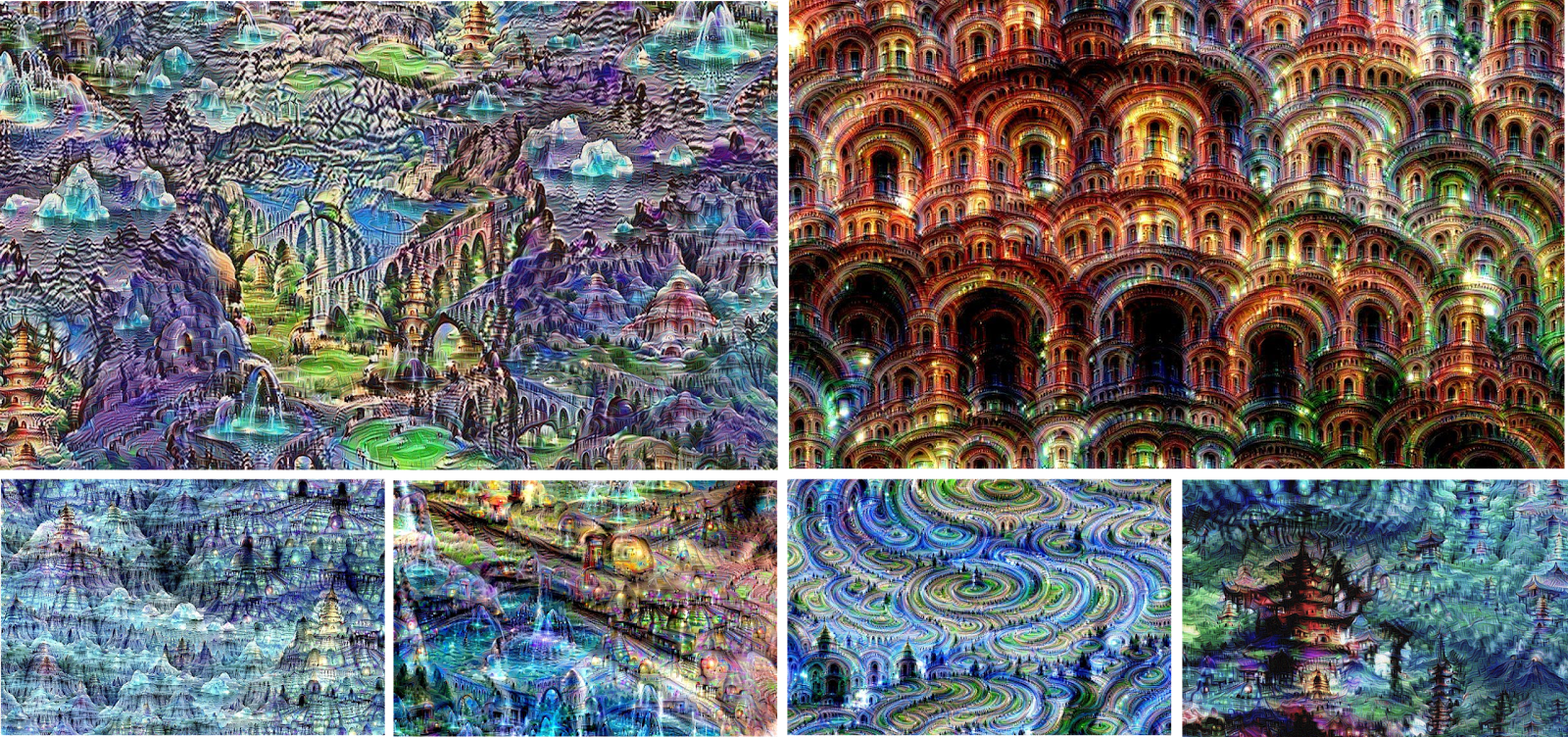Neural net “dreams”— generated purely from random noise, using a network trained on places by MIT Computer Science and AI Laboratory. See our Inceptionism gallery for hi-res versions of the images above and more (Images marked “Places205-GoogLeNet” were made using this network).

The techniques presented here help us understand and visualize how neural networks are able to carry out difficult classification tasks, improve network architecture, and check what the network has learned during training. It also makes us wonder whether neural networks could become a tool for artists—a new way to remix visual concepts—or perhaps even shed a little light on the roots of the creative process in general.

We have published our latest review, on methods to infer horizontal gene transfer, in Wikipedia. It was peer-reviewed and it simultaneously appeared in PLOS Computational Biology. After our review on approximate Bayesian computations published two years ago, this is our second contribution using an exciting new format called “Topic Page”. In this post, I reflect on our motivation and experience as Topic Page authors. The difficult relationship between academia and Wikipedia Academia has mixed feelings about Wikipedia. Although many academics—and certainly many students—consult Wikipedia frequently, I’d venture to say that most remain reluctant to cite Wikipedia or admit relying on it otherwise. As for academics contributing to Wikipedia, things are even worse. As a result, the quality of Wikipedia articles on scientific topics is often quite poor. I think there are two main reasons for this reluctance to contribute. First, the lack of clear authorship and therefore credit makes it difficult for scientists to get recognition for contributing to Wikipedia. Given the intense competitiveness of contemporary science, this is more than a vanity issue; recognition is tightly coupled with funding and job success—i.e. survival in the profession. But perhaps just as importantly, many scientists are unfamiliar with Wikipedia’s conventions and practices and are thus (rightly!) concerned that their contributions might be “diluted” by further edits by others or even flat out turned down. I know of several disgruntled people who have given up on editing Wikipedia because of such bad experiences. Simson Garfinkel provides an illuminating account of this sort of tensions in this article: “I have attempted to retire from directing films in the alternative universe that is the Wikipedia a number of times, but somebody always overrules me,” Lanier wrote. “Every time my Wikipedia entry is corrected, within a day I’m turned into a film director again.” Since Lanier’s attempted edits to his own Wikipedia entry were based on firsthand knowledge of his own career, he was in direct violation of Wikipedia’s three core policies. He has a point of view; he was writing on the basis of his own original research; and what he wrote couldn’t be verified by following a link to some kind of legitimate, authoritative, and verifiable publication. For the tertiary source Wikipedia aims to be, these core policies are entirely reasonable but it’s easy to imagine situation where they might frustrate some contributors. Wikipedia’s tremendous impact It’s however worth considering the upsides of contributing to Wikipedia. For all the obsessions many of us have about publishing articles in generalist journals with broad readership, the lack of interest in Wikipedia feels like a missed opportunity. Consider the wikipedia page on Phylogenetics. It was consulted over 50,000 in the last 3 months alone. This is over twice as much as the median number of views of papers published in, say, the 17 Oct 2013 issue of Nature in a quarter of the time (as it happens, this particular issue has “impact metrics” as its cover story…). PLOS Topic Pages Fortunately, the good folks at PLOS Computational Biology have worked out a great solution to this conundrum: the “Topic Page”. In short, authors contribute Wikipedia-style articles on topics not or only poorly covered in Wikipedia. These get peer-reviewed and published in the journal with attribution, a DOI, and all the bells and whistles that come with journal articles. But in addition, the page gets incorporated into Wikipedia, where it starts a new life. This format solves the problem discussed above. Authors get credit for their work in a way that fits well to existing structures. There is a permanent record of the contribution, indexed in scholarly databases such as PubMed, Google Scholar, etc. The contribution benefits from additional feedback from the peer-review and editorial process. And, perhaps most importantly, the authors can relinquish control over their work—for better or worse—with the reassurance that an unadulterated version of their work will remain available no matter what. Our experience publishing Topic Pages So far, we have published two Topic Pages: one on Approximate Bayesian Computations (paper, peer-reviews, Wikipedia page and one on inferring horizontal gene transfer (paper, peer-reviews, Wikipedia page). We’ve been pleasantly surprised by the excellent reception of the ABC article. It has been viewed over 26,000 times on the PLOS site alone. It’s also consulted a few thousand times every month on Wikipedia. Remarkably, since the article was publicly accessible while we were drafting it on the PLOS Topic Page wiki, it had already accumulated over 10,000 views even before publication (see counter at bottom of this page). It was also picked up by a prominent’s statistician’s blog. But just as importantly, the editorial process itself was great. Editing the manuscript on the PLOS Topic Page wiki provided a natural environment for collaborative writing. The wiki-based, open peer-review process yielded constructive and timely reviews (we could start addressing referee reports as they rolled in!). Our editor Daniel Mietchen was helpfully hands-on and did a substantial number of edits directly on the manuscript itself. The only caveat I can think of is that the neutral, factual, impersonal, intemporal style of Wikipedia articles is quite different from the type of review articles I am otherwise used to. This is definitely not the right outlet for opinion-type pieces! On the other hand, this format is great for student work. In fact, both of our Topic Pages started as student assignment in my course Reviews in Computational Biology. That being said, although the course gave the initial impetus, in both cases extensive additional work (and the involvement of additional co-authors) was required to get them published. What happened since? As it’s been two years since we published the ABC review, we can start to discern some outcomes. The Wikipedia version underwent 46 changes, all minor modifications or additions (typo corrections, additional links and “Wikifications”, additional entries in the list of relevant software packages, attempts to sneak in one’s own contributions, … the usual stuff). It is also gratifying to see our work appearing as first hit in Google. Since the publication in early 2013, it’s already been cited over 50 times. Way of the future In conclusion, the Topic Page is a great format. I am surprised that only eight Topic Pages have been published thus far, but perhaps there is still a lack of awareness about the format. I hope that this blog post will inspire some readers to improve Wikipedia by contributing a Topic Page. We are certainly thinking of our Topic Page number three… References Ravenhall M, Škunca N, Lassalle F, & Dessimoz C (2015). Inferring horizontal gene transfer. PLoS computational biology, 11 (5) PMID:...

Children who benefit from a good memory are much better at covering up lies, researchers from the University of Sheffield have discovered. Experts found a link between verbal memory and covering up lies following a study which investigated the role of working memory in verbal deception amongst children. The study saw six to seven year old […]...

Scientists have successfully increased the infiltration of immune cells into tumors, thus inducing the immune system to block tumor growth. In a new article, the scientists show that, in combination with existing immunotherapies, this process efficiently destroys cancer cells.