• N is the number of ALS iterations, D is the number of latent factors. The experiments have been conducted on a 16 node cluster. 
• We start GL as mpirun -hostfile ~/hostfile -x CLASSPATH ./als –ncpus=16 --matrix hdfs://host001:19000/user/netflix --D=$LATENT_FACTOR_COUNT --max_iter=$ITER_COUNT --lambda=0.065 --minval=0 --maxval=5 
• To run mahout ALS, we use the factorize-netflix.sh script under the examples directory. It should be run as ./factorize-netflix.sh /path/to/training_set/ /path/to/qualifying.txt /path/to/judging.txt 
• In our test cluster we have 16 machines each with 64GB of memory, 2 CPUs (Intel(R) Xeon(R) CPU E5-2670 @ 2.60GHz [8 cores each]) and 4 x 1 TB HDDs. The machines communicate over a 10Gb Ethernet interconnect. 
• The Netflix dataset has been splitted into 32 equally sized chunks and then put into HDFS.

What is pyvideo.org

pyvideo.org is an index of Python-related conference and user-group videos on the Internet. Saw a session you liked and want to share it? It's likely you can find it, watch it, and share it with pyvideo.org.

Status

• Videos for PyCon US 2013 are still going up. There are 115 posted and live now. There are around 30 that are waiting for presenters to look at the metadata and tell Carl whether the metadata is good or not. More on that later.

• Several new people submitted patches to richard! Several of the patches were fixes to broken things they saw on pyvideo.org. I've applied the fixes to the site directly, but have been waiting on making any non-critical updates to the site until after things have cooled off. I think I'll do a site update in the next week or so.

• PyData 2013 was recorded. When videos are posted, they'll be in the PyData category. I don't know what the posting schedule is.

• I was contacted a couple of times by the inimitable Montréal Python to post their videos. They're going to test out steve which is the tool I've been writing for the last 6 months to make it possible for other folks to generate the video metadata needed by pyvideo.org.

  I eagerly look forward to their progress and to their videos getting on the site.

  If it works out well, I'll blog more about steve and look for volunteers to use steve to generate the video metadata for the ever increasing backlog.

• Several people are gittip'ing me. It's not a lot of money, but that and the many emails I've gotten over the last few weeks about the site have been really great. I work on pyvideo.org in my free time of which I don't have a lot. It's nice to know that prioritizing pyvideo.org work over other things helps you.

That's the gist of things!

Most of the PyCon US 2013 videos that aren't live are waiting for presenters to tell Carl at NextDayVideo (carl at nextdayvideo dot com) whether the metadata is good.

• If you see your name on this list and you've told Carl the metadata is fine already, please send him a friendly reminder.
• If you see your name on this list and you haven't told Carl anything, please send him a "yes, this is great!" or the list of things you need corrected.
• If you see a friend on this list, tell your friend to do one of the above.

I'll update this list as I'm aware of changes. However, I don't work for NextDayVideo, so it's entirely possible my list is not current and/or there are errors. If so, please let me know.

Here's the list (last updated 2013-04-03 9:11am -0400):

• Digital signal processing through speech, hearing, and Python -- Mel Chua
• IPython in-depth: high-productivity interactive and parallel python -- Fernando Perez, Brian Granger, Min RK
• Faster Python Programs through Optimization -- Mike Müller
• Pyramid for Humans -- Paul Everitt
• Python beyond the CPU -- Andy Terrel, Travis Oliphant, Mark Florisson
• Code to Cloud in under 45 minutes -- John Wetherill
• Learn Python Through Public Data Hacking -- David Beazley
• A Gentle Introduction to Computer Vision -- Katherine Scott, Anthony Oliver
• Documenting Your Project in Sphinx -- Brandon Rhodes
• Contribute with me! Getting started with open source development -- Jessica McKellar
• Intermediate Twisted: Test-Driven Networking Software -- Itamar Turner-Trauring
• Gittip: Inspiring Generosity -- Chad Whitacre
• Rethinking Errors: Learning from Scala and Go -- Bruce Eckel
• The Magic of Metaprogramming -- Jeff Rush
• You can be a speaker at PyCon! -- Anna Ravenscroft
• sys._current_frames(): Take real-time x-rays of your software for fun and performance -- Leonardo Rochael
• Planning and Tending the Garden: The Future of Early Childhood Python Education -- Kurt Grandis
• powerful pyramid features -- Carlos de la Guardia
• Python for Robotics and Hardware Control -- Jonathan Foote
• Copyright and You -- Frank Siler
• Chef: Automating web application infrastructure -- Kate Heddleston
• Numba: A Dynamic Python compiler for Science -- Travis Oliphant, Siu Kwan Lam, Mark Florisson
• Integrating Jython with Java -- Jim Baker, Shashank Bharadwaj
• Iteration & Generators: the Python Way -- Luciano Ramalho
• ApplePy: An Apple ][ emulator in Python -- James Tauber
• Distributed Coordination with Python -- Ben Bangert
• Become a logging expert in 30 minutes -- Gavin M. Roy
• PyNES: Python programming for Nintendo 8 bits -- Guto Maia
• Purely Python Imaging with Pymaging -- Jonas Obrist
• Namespaces in Python -- Eric Snow

[Comments]

A Programmer’s Guide to Data Mining – The Ancient Art of the Numerati by Ron Zacharski.

From the webpage:

Before you is a tool for learning basic data mining techniques. Most data mining textbooks focus on providing a theoretical foundation for data mining, and as result, may seem notoriously difficult to understand. Don’t get me wrong, the information in those books is extremely important. However, if you are a programmer interested in learning a bit about data mining you might be interested in a beginner’s hands-on guide as a first step. That’s what this book provides.

This guide follows a learn-by-doing approach. Instead of passively reading the book, I encourage you to work through the exercises and experiment with the Python code I provide. I hope you will be actively involved in trying out and programming data mining techniques. The textbook is laid out as a series of small steps that build on each other until, by the time you complete the book, you have laid the foundation for understanding data mining techniques. This book is available for download for free under a Creative Commons license (see link in footer). You are free to share the book, and remix it. Someday I may offer a paper copy, but the online version will always be free.

If you are looking for explanations of data mining that fall between the “dummies” variety and arXiv.org papers, you are at the right place!

Not new information but well presented information, always a rare thing.

Take the time to read this book.

If not for the content, to get some ideas on how to improve your next book.

Concurrent and Parallel Programming by Joe Armstrong.

Joe explains the difference between concurrency and parallelism to a five year old.

This is the type of stark clarity that I am seeking for topic map explanations.

At least the first ones someone sees. Time enough later for the gory details.

Suggestions welcome!

from mpl_toolkits.basemap import Basemap
from pylab import *
import twitter_geo

# setup Lambert Conformal basemap.
m = Basemap(width=400000,height=400000,projection='lcc',resolution='f',lat_0=55.5,lon_0=13)
m.bluemarble() #background
m.drawcoastlines() #coastlines

# get some geo data from Twitter
geo = '55.583333,13.033333,100km' #Malmo, Sweden
tweets = twitter_geo.parse(twitter_geo.search(geo=geo))

for t in tweets:
    coords = t[2]['coordinates']
    x,y = m(coords[1],coords[0]) #project to map coords
    plot(x,y,'ro')

show() #you might not need this

from numpy import *
import cv

capture = cv.CaptureFromFile('skyline.mov')
frames = []
for i in range(100):
    img = cv.QueryFrame(capture)
    tmp = cv.CreateImage(cv.GetSize(img),8,3)
    cv.CvtColor(img,tmp,cv.CV_BGR2RGB)
    frames.append(asarray(cv.GetMat(tmp))) 
frames = array(frames)

from scipy.linalg import rq

from scipy.linalg import qr

def rq(A): 
 Q,R = qr(flipud(A).T)
 R = flipud(R.T)
 Q = Q.T 
 return R[:,::-1],Q[::-1,:]

# factor first 3*3 part of P
K,R = rq(P[:,:3])

# make diagonal of K positive
T = diag(sign(diag(K)))

K = dot(K,T)
R = dot(T,R) #T is its own inverse

from numpy import *

def adjacency_matrix(im,connectivity=4,sparse=False):
 """ Create a pixel connectivity matrix with
  4 or 8 neighborhood. If sparse then a dict is
  returned, otherwise a full array. """

 m,n = im.shape[:2]

 # center pixel index
 c = arange(m*n)
 ndx = c.reshape(m,n)

 if sparse:
  A = {}
 else:
  A = zeros((m*n,m*n))

 if connectivity==4: # 4 neighborhood
  hor = roll(ndx,1,axis=1).flatten() # horizontal
  ver = roll(ndx,1,axis=0).flatten() # vertical
  for i in range(m*n):
   A[c[i],hor[i]] = A[hor[i],c[i]] = 1
   A[c[i],ver[i]] = A[ver[i],c[i]] = 1

 elif connectivity==8: # 8 neighborhood
  hor = roll(ndx,1,axis=1).flatten() # horizontal
  ver = roll(ndx,1,axis=0).flatten() # vertical
  diag1 = roll(roll(ndx,1,axis=0),1,axis=1).flatten() # diagonal
  diag2 = roll(roll(ndx,1,axis=0),1,axis=0).flatten() # diagonal
  for i in range(m*n):
   A[c[i],hor[i]] = A[hor[i],c[i]] = 1
   A[c[i],ver[i]] = A[ver[i],c[i]] = 1
   A[c[i],diag1[i]] = A[diag1[i],c[i]] = 1
   A[c[i],diag2[i]] = A[diag2[i],c[i]] = 1

 return A

from pylab import *

im = random.random((10,10))
A = adjacency_matrix(im,8,False)

figure()
imshow(1-A)
gray()
show()

1. U. Bag ̆cı and E. Erzin, "Boosting classifiers for music genre classifi- cation," in Proc. 20th Int. Symp. Comput. Inform. Sci. (ISCIS'05), Istanbul, Turkey, Oct. 2005, pp. 575-584.
2. U. Bagci and E. Erzin, "Inter genre similarity modeling for automatic music genre classification," in Proc. IEEE Signal Process. Comm. Apps., pp. 1-4, Apr. 2006.
3. U. Bagci and E. Erzin, "Inter genre similarity modeling for automatic music genre classification," in Proc. DAFx 2006.
4. U. Bagci and E. Erzin, "INTER GENRE SIMILARITY MODELLING FOR AUTOMATIC MUSIC GENRE CLASSIFICATION" arXiv:0907.3220v1, 2009.

  % create initial models (mixture of Gaussians classifier)
  W = mogc(traindataset,numGaussians);
  % classify
  results = traindataset*W;
  predictedLabels = results*labeld;
  % find those frames that are wrongly classified
  idx_wrong = ~(predictedLabels == traindataset.nlab);
  
  % create new dataset from those wrongly classified
  newlabels = traindataset.nlab;
  newlabels(idx_wrong) = 0; % this is the IGS class
  traindataset = dataset(traindataset.data,newlabels);
  traindataset = setprior(traindataset,0);
  % create final models
  W = mogc(traindataset,numGaussians);
  
  % test
  results = testdataset*W;

    sumlogpost = -Inf*ones(numclasses,1);
    % compare posteriors of each class to those of IGS model
    for jj=1:numclasses
      posteriorsforthisclass = posteriors(:,jj+1);
      % find those that have posteriors above that of IGS
      idx = (posteriorsforthisclass > posteriors(:,1));
      numframestoconsider(jj) = sum(idx);
      if numframestoconsider(jj)
        sumlogpost(jj) = sum(log(posteriorsforthisclass(idx)))/numframestoconsider(jj);
      end
    end
    [~,pred] = max(sumlogpost);

1. there are common properties among music genres, for instance, "similar types of instruments with similar rhythmic patterns";
2. the nature of some of these common properties is such that bags of frames of features (BFFs) encapsulate them;
3. this means we should expect poor automatic genre recognition using BFFs if these common properties are quite prevalent among the classes; (or, that music genres have common properties is to some extent responsible for their ambiguousness;)
4. we can model the common properties of a set of music genres by combining the features of frames that are misclassified in each genre;
5. we can model the non-common properties of each of a set of music genres by combining the features of frames that are correctly classified in each genre;
6. with these models, we can thereby ascribe a confidence that any given frame encapsulates common properties, and thus whether to treat it as indicative of genre or not.

1. there are common properties among the classes in dataset X;
2. the nature of some of these common properties is such that our features encapsulate them;
3. this means we should expect poor automatic recognition using these features if the common properties are quite prevalent among the classes;
4. we can model the common properties of our classes by combining the features that are misclassified in each genre;
5. we can model the non-common properties of each of our classes by combining the features that are correctly classified in each class;
6. with these models, we can thereby ascribe a confidence that any given set of features (an observation) encapsulates common properties, and thus whether to treat it as indicative of a class or not.

• Reproducible Research ( implementations featured on Nuit Blanche)

• Nobody Cares About You and Your Algorithm
• These Technologies Do Not Exist
• The Big Picture in Compressive Sensing 
• The Advanced Matrix Factorization Jungle
• Nuit Blanche blog entries featuring papers with attendant code implementations.

Liked this entry ? subscribe to Nuit Blanche's feed, there's more where that came from

Edit 21 Jan 2013: added “Example 3″ to the title.

Introduction

I’m going to jump right in and imagine that we have a known plant which we wish to control using P, PI, or PID. I’m going to assume that you have some idea what those are. We’ve seen proportional (P) control, where the control signal is proportional to the error. Integral control has a signal which is proportional to the integral of the error, and derivative control a signal which is proportional to the rate of change (the derivative) of the error. Proportional control is always used in conjunction with integral, hence PI. Although derivative control can be used with only proportional, in process control we generally use both integral and proportional with it, hence PID. We’ll talk more about them in subsequent posts, but for now I want to show you two ways to get the required parameters. They may not always be very good values, but they’ll be better than in the ballpark. At the very least, they are good starting values for further investigation.

Oh, I am aware that Mathematica® version 9 has new capabilities for tuning controllers – but let me write about what I know, using version 8.

My plant is a 3rd-order transfer function… as usual, rules are a convenient way to specify things:

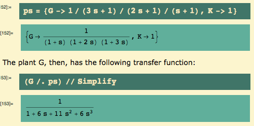
Bequette – this is Example 5.3 (p. 174) and Example 6.1 (p. 199) from Bequette’s “Process Control: Modeling, Design, and Simulation”, Prentice Hall 2003. He used the Routh criterion to decide that the ultimate gain was 10: that’s on the verge of instability. Let’s take a look – that is, I’m about to show you what the ultimate gain means.

I set a new parameter value for K, namely K = 10, the alleged ultimate gain.

The closed loop transfer function (y) is…. and the time-domain response to a unit step function is…

Let’s get the control effort transfer function u, too… and the time-domain behavior:

Here’s my usual first plot: step function in silver (or whatever it is), system response in black, scaled control effort (c1/K) in gold:

OK, we see steady-state oscillations in response to a unit step input. Make K slightly greater, and the oscillations will grow; make K slightly smaller and the oscillations will get smaller. We are on the edge of instability, just as advertised.

I should also show you the actual control effort:

We would like to know the period of these output oscillations. It looks like it is slightly above 6… there’s a minimum just before 7, and the next one is just after 13 – look at the previous graph… that’s why I scale the control effort, so the output is not compressed.

We could use calculus to find them…. If we were looking at a paper recording, we might be able to measure them, but in this case we have an explicit equation for the solution, so let’s go ahead and do calculus. Here’s the first derivative of the output… set it to zero.

Let’s find solutions near 7 and 13…

We could also back up, and instead of finding the ultimate gain by the Routh criterion, we could have found it by simulation. I’ve shown you simulation before, so I won’t do it this time. If, instead of having a math model, you were in the control room playing with parameters, you’d be using the system itself to do a simulation… and the operators would be planning to kill you for bringing the system to the edge of instability.

The bottom line, however, is that we now have two parameters, called the ultimate gain and the ultimate period. There are some simple tuning rules – choices of P, PI, and PID settings – which are based on these two parameters.

But first let me show you the right way to get the ultimate gain and ultimate period, if you have a quantitative model. Everything else in this post is straight-forward, I hope, but this trick is not, at least to me.

We return to our initial system (K = 1):

And here’s the open loop Bode plot:

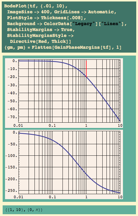
The gain margin is 10 – gee, that’s the ultimate gain Bequette found! It occurs at a frequency of 1 radian/second.

Given a frequency f in radians/second, we find the period from P f = 2 pi. This crossover frequency is 1, so the corresponding period is

… and that is the ultimate period we computed by finding two consecutive minima.

Don’t ask me why it works, I don’t understand it yet. But I have more than one book telling me it’s not an accident. This, as far as I’m concerned at this point, is the main use of the gain margin. There’s absolutely no reason to simulate the math model and estimate these numbers: they can read off the gain margin. If you have a math model.

Now save these:

Now that we have Pu and ku, there are some rules for setting the parameters of P, PI, and PID controllers. But while I have the default K = 1, let’s see how the uncontrolled plant responds to a unit step. I get the closed loop transfer function and then the inverse Laplace transform:

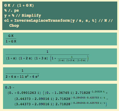
Here’s the output and the input (black and silver resp.)

Well, except that it’s nowhere near 1 – i.e. we have offset – it had a pretty gentle response, without wild swings.

With a PID controller, we have plant… and controller…

We see three parameters: an overall gain kc, and two time constants, and . The is multiplied by s – which says that’s the Laplace transform of a derivative… and the is coupled with a 1/s – which says that’s the Laplace transform of an integral. What I’m going to show you is two sets of rules for getting from the ultimate gain and the ultimate period to values of kc, , and .

The first set of rules is called Ziegler-Nichols; the second is called Tyreus-Luyben.

Let’s go.

Ziegler-Nichols with P, PI, PID

First, let’s try the Ziegler-Nichols rules.

P-only control

To get P-only control, we set ->0 and -> .

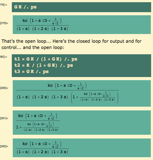
Here are the closed loop transfer functions for output and for control… and, since I will want it later, the open loop transfer function, too:

The Z-N rule for P-only control is to set kc = .5 ku. (Parts of the following rule are redundant, because I’ve already set and , but I like having a complete rule anyway.)

and the closed loop for control becomes

We get the time-domain responses by taking inverse Laplace transforms…

And we plot the input (step function in “silver”), output (black), and scaled control effort (gold):

Not only does it take a long time to settle, but there is offset. As for the long settling time… K = 1 got there quickly, K = 10 was on the edge of instability, so K = 5 should have decaying oscillations. OK?

(And if you’re not used to seeing offset with P-only control… remember that the use of transfer functions requires that we use deviation variables: all our initial conditions are zero, in these variables. That is, for example, we’re not using the actual liquid level in a tank – we’re using the deviation from the set point. To hold the system at a value other than zero requires a constant nonzero control effort… so the response is nonzero, but not necessarily 1.)

For the record, here’s the unscaled control effort (gold):

Lastly, I want to see the open loop Bode plot, and compute the phase margin:

The phase margin is 25° – a little too jittery, as we saw.

PI control

To get PI control, we set ->0.

Here are the closed loop transfer functions for output and for control… and the open loop transfer function for later:

Note that kc has changed a little: instead of .5 we have .45 . What this says is that the control modes interact: they should not be set independently of each other…once we add integral control to proportional control, we change the value of the proportional control… and we’ll change both of them again when we add derivative control.

The closed loop transfer function for output becomes.. and we know the ultimate gain ku and ultimate period Pu:

The closed loop for control becomes

The open loop transfer function becomes

The time-domain responses become:

And here’s the usual plot, including scaled control effort:

It still takes a long time to settle, but the offset is gone.

After all, that’s one of things integral control does for us: it eliminates offset. I should point out that we don’t always care about offset: level control for surge tanks is the best example where we do not care to hold the level at exactly 50%. In fact, to do so would defeat the purpose of a surge tank, and we might as well replace it by a pipe – what goes out is exactly what comes in.

Here’s the unscaled control effort:

And here’s the open loop Bode plot:

This quantifies what we saw: that the output is more jittery than P-only control.

PID control

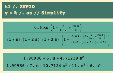
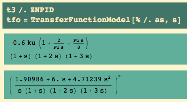
To get PID control, we keep all three PID parameters:

Here are the closed loop transfer functions for output and for control… and, as usual, the open loop transfer function for later:

This time kc is greater than .5, is smaller than for PI.

The closed loop transfer function for output becomes.. and we know the ultimate gain ku and the ultimate period Pu:

and the closed loop transfer function for control becomes

The open loop transfer function becomes

The time domain responses…

… and the usual plot:

As usual, here is the unscaled control effort:

The open loop Bode plot is

That phase margin of 29 is… marginal, at best – go ahead, grimace and hate me; still too jittery.

Let’s take a look at the three output responses:

I used panels 3-5 from the following, so orange is P, brown is PI, and yellow is PID. Alternatively, the orange must be P because it has offset, so PID should be yellow.

Anyway, we see that P has offset… PI does not, but it takes longer to settle down than P did… PID settles down much faster than the other two, and has no offset, but it still swings wildly at first (that overshoot is just over 40%.)

Tyreus-Luyben with PI, PID

Now I try the Tyreus-Luyben rules. Like the Ziegler–Nichols, they use ultimate gain ku and ultimate period Pu. For P-only control, they are the same.

PI control

To get PI control, we set ->0.

Here are the closed loops for output and for control… and, of course, the open loop transfer function:

The T-L rule for PI control is

The closed loop for control becomes

The open loop becomes

The time-domain responses are…

Here is the usual plot showing input, output (black), and scaled controller effort:

Settles faster, and the offset is gone.

Here’s the unscaled control effort:

Here’s the open loop Bode plot:

OK, we finally have a phase margin (39°) which is greater than 30°: this choice of parameters is OK by that criterion.

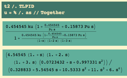
PID control

To get PID control, we need all three PID parameters:

The T-L rule for PID control is

and the closed loop transfer function for control becomes

The open loop transfer function becomes

Here are the time-domain responses:

Here is the usual plot…

Here’s the unscaled controlled effort:

Here, as usual, is the open loop Bode plot:

Even better than the PI control: a not-too-large phase margin.

Now let’s compare things. Here are the two PI controls:

The T-L has significantly less wildness than the Z-N: the overshoot is less and the settling time is less.

Here are the two PID controls:

The T-L has significantly less overshoot, but it does take a little longer to get close to its final value. That probably corresponds to a phase margin close to 60°.

I shouldn’t even think of putting all 5 controllers on one graph….

…though they look better if I shorten the time, except that it is no longer clear that P-only has offset:

Recall the colors in order, orange (3) thru dark gray (7): so, orange, brown, and yellow are Z-N P, PI, and PID; light and dark gray are T-L PI and PID.

Summary

Here are the Ziegler-Nichols rules:

Here are the alternative Tyreus-Luyben rules:

These rules require that we determine the ultimate gain and the ultimate period… and we saw how to get them from the open loop Bode plot, specifically from the gain margin and the frequency at which it occurs.

We saw the effect of these rules on a particular plant, and we also checked the phase margin for each choice of control method and parameters.

As you might expect, I would tend to go with the Tyreus-Luyben rules.

There’s something I forgot to do when I looked at PID tuning: I meant to look at the Bode plots for the controllers, literally to see what they do individually. In addition, I’m going to mention real derivative control; I’ve long known that the simple PID includes “ideal” derivative control, but I only just realized just how unrealistic it is.

It’s probably just as well that this end up in a separate post.

Let’s just dive in to Bode plots.

PID with Ziegler-Nichols rules

Recall our plant… first the definition, then the resulting transfer function.

We found, by looking at the gain margin for the open loop Bode plot of the plant that the ultimate gain and ultimate period were 10 and :

Ah, I need to say – and to add a comment to the previous post – that my lack of understanding is not complete. If we accept the dictum that the gain margin tells us how much the gain can be multiplied before the system goes unstable, then to that extent, it makes sense that the gain margin tells us the ultimate gain. My lack of understanding then focuses on the question: why is the gain margin computed at a phase of -180° ? I’m not setting the phase to that when I hit the system with a unit step. Perhaps one argues that the unit step includes a component at a phase of 180°…. I’m sure I’ll understand it someday.

Anyway, we know in practice that the ultimate gain and ultimate period are found from the gain margin of the open loop Bode plot of the plant.

With PID control, we redefine K… and get the general open loop transfer function for our given plant:

The Z-N settings for PID control are:

The open loop for plant and controller becomes

Here’s the plant alone:

I also want the complete PID controller by itself. Incidentally, the last thing I did was factor the controller.

I should emphasize something that I never noticed before: the PID controller is improper, because the numerator is of higher degree (2) than the denominator (1). The problem is the “ideal” derivative term… sometime soon I will have to show you “real” derivative transfer functions (there’s more than one).

Here’s the open loop Bode plot for the uncontrolled plant…

We’ve seen it before, of course: the {1,10} told us the gain margin was 10 – the ultimate gain – at a frequency of 1 – hence a period of 2 / 1 = 2 – the ultimate period.

The open loop Bode plot for the fully controlled plant is – again…

We’ve seen this before, too: the Z-N rules lead to a phase margin of 29°, which is right on the edge of acceptability (30°).

The plant G and the controller K are in series, so we may look at all three (G, K, GK)on one open loop Bode plot. Blue is the plant G, red is the PID controller K, and gold is the controlled plant G K. We see that the controller has a minimum, and increases the amplitude plot everywhere else. Looking at the gold curve versus the blue curve in the amplitude plot, we see that at low frequencies, the controller causes the amplitude to rise; at high frequencies it causes the amplitude to fall off less rapidly.

Now we could get the P-only part of the controller K (but I won’t actually do anything with it):

We saw in an earlier post how to break down a transfer function as a product of terms. Unfortunately, a PID controller is not a product of terms in that sense, but a sum; we cannot write it as a product of P, PI, PD. (That was why I factored it earlier; just to show that it wasn’t product of its components.)

Maybe, just for completeness, I should extract the ID part of the controller – at least, as far as possible; I can’t actually do it because ID without P would cancel the s in the numerator with the s in the denominator. That is, I can factor out the “6″, but I can’t completely eliminate the P term; all I can do is set P = 1 here (by setting ku = 1/.6). Here’s what I get if I do that:

And that’s what I want to do for PI and PD: set their P terms to 1…

Here’s the PI part of the controller, using the ZNPID settings but P = 1:

And here’s the PD part:

Incidentally, looking at the PI and PD controllers, we see that the PD controller itself is improper, while the PI controller is semi-proper (same degree in numerator and denominator). This is why I said earlier that the problem was in the “ideal” derivative control.

Let’s look at the PI and PD controllers that we extracted:

The blue curve is the PD controller: it increases the amplitude at high frequencies; we might say it reacts to noise. The red curve is the PI controller; it increases the amplitude at low frequencies.

Where are the break point frequencies? Look for the zeroes in these cases.

So, the break points are at .32 and 1.27 . The region between them is relatively unaffected. This tells us that the break point frequency for PD should be higher than the break point frequency for PI. (We’ll come back to this.)

Now let us add the PID controller to them:

I want to spread out the break points of the two controllers. Let’s put the PI breakpoint at .1 and the PD break point at 10. Note that I have to invert both numbers: -> .1 and -> 10. (Of course I have to invert: .) Here’s the resulting PID controller:

We see that there was some interaction… the PI breakpoint isn’t exactly at 10, and the PD breakpoint isn’t exactly at .1 . Here’s the Bode plot for the resulting PID controller:

Now that we have been reminded that the breakpoints are approximate inverses of the time constants and , we can recall the Z-N PID rules:

Yes, they show smaller than , by a factor of 4… but that means the breakpoint from the PD portion is larger than the breakpoint for the PI portion.

I should also look at Tyreus-Luyben rules.

Recall our plant with PID control:

The T-L settings for PID control are:

We see that is bigger than . This is in line with what we learned looking at the Z-N rules: we end up with a smaller breakpoint frequency for PI than for PD.

The open loop for plant and controller becomes, with T-L PID settings:

The PI part of it… but I use the T-L PID settings – and divide by .454545 rather than by .6 to get P = 1:

And here’s the PD part of it:

I also want the PID controller by itself (i.e. with P = 1):

Here’s the open loop Bode plot for the controlled plant:

We’ve seen this before, too: the T-L rules lead to a phase margin of 54°.

Let’s look at the PI and PD controllers alone:

The blue curve is the PD controller: it increases the amplitude at high frequencies; the red curve is the PI controller, it increases the amplitude at low frequencies.

We see immediately that the breakpoint frequencies have been separated more than by the Z-N rules.

Exactly where are the break point frequencies?

So, the break points are at .07 and 1. The region between them is not affected.

Now lets add the PID controller to the PD and PI curves:

As before, blue is PD and red is PI, and gold is PID.

Just for the fun of it, let’s see what happens if we interchange the values of and , using our values of 10 and .1 . Here’s the PD transfer function, which has a zero at -.1 .

Now set only -> .1 … and we get a zero at 10 …

Here’s the two of them together:

And here’s the corresponding PID controller…

And here’s the open loop Bode plot of that PID:

I’d say that’s a rather striking difference.

Let’s look at all three.

Do you begin to believe that the PID is not the product of the PI and the PD? I suppose I could simply compute the product… well, with transfer functions, I connect them in series…

And here’s the product PI PD overlaid on the actual PID:

OK? PID ≠ PI PD in series.

Summary

We’ve seen what a PI and a PD controller look like…

We’ve discovered that we want > in a PID controller.

We’ve discovered that although we can factor out the P ≠ 1 term from a PID controller, we cannot then factor the remainder into PI PD or into I D.

We’ve discovered that ideal derivative control leads to an improper – physically unrealizable – controller, in both PD and PID. We should look at real derivative control – even though the overwhelming majority of chemical process analyses use ideal derivative control!

But we’ll not look at that today.

The EOQ (Economic Order Quantity) formula is a deceptively simple model. It comes from Zipkin’s “Foundations of Inventory Management” (Irwin/McGraw-Hill, 2000, 0-256-11379-3) and it is the very first model in the book. It was first published 100 years ago, in 1913 – the model, not the book!.

When all is said and done, it’s a simple application of freshman calculus.

Imagine that we sell or use up one product, at a known constant rate . Periodically, we order more of this product, to replenish our inventory I(t). Further, there is a known constant lead time L – between when we place an order and when we receive it (actually, when we can sell or use it, so this includes unloading and storing). If our inventory will go to zero at t = T, then, at the very latest, we must place an order at T – L:

Since we assume that the demand and the lead time L are constants, we can safely place our order at exactly T – L. A more realistic model would allow for uncertainty in and L. Oh, of course, I am assuming that running out of inventory is not acceptable: we want to always meet demand.

This means that if we order q, our inventory jumps from 0 to q upon delivery of our order.

Now, there are a lot of caveats for this model. For example… what if we’re only open for 8 hours a day, 5 days a week? Then this model would require us to count only the time we’re open, to assume that lead time does not include the weekend days, and that deliveries occur while we’re open…. But let me stay with this first model.

In addition to inventory on hand at time t, I(t), we also define inventory on order IO(t) and inventory position IP(t) as their sum. That is, we have

a constant rate of demand (quantity/time)
L a constant lead time between placing an order and receiving it
q order quantity
I(t) inventory at time t
IO(t) inventory on order at time t
IP(t) inventory position at time t, where

IP(t) = I(t) + IO(t).

What we want to know is how much to order and often to order it. Yes, those are related questions. The key is that if we place an order for q once during the time required to completely deplete our inventory, then we are placing an order every

.

(The time between orders, one cycle, is , so the frequency of orders (the order frequency OF) is the inverse.)

During that cycle, the average inventory is .

Now, what’s it cost to do this? We can break the costs into three different kinds:

k fixed cost to place an order
c variable cost to place an order
h cost to hold one unit of inventory for one unit of time.

(So the cost of inventory I(t) is h I(t), and the average cost of inventory in one cycle is h q/2.)

The total cost of an order q placed every cycle, then, is

C(q) = order cost + holding cost

hence the order cost, the holding cost, and the total cost are:

It’s crucial that the holding cost increases with q, while the order cost decreases with q.

I need some numbers.

Zipkin’s numerical example is of paper for the copy machine(s):

usage (demand) is 8 boxes/week at $25 per box.
handling (on our end) and shipping is $80 + $50.
the shipment takes a week to arrive.
keeping inventory organized is $1.10 per week.
Financing is 15% per year.
We order 2 weeks worth of supplies (16 boxes) with each order.

(That finance charge is applied to the cost of each box. At least, that’s how I think of it.)

That is,

= 8
k = 80 + 50
L = 1
c = 25
q = 16
h = 1.10 + .15/52

and that in turn is (omitting q):

With these numbers our average order cost, holding cost, and total cost become – as functions of q

We can plot them over an indicative range, q goes from 10 to 100:

The red line is the linear holding cost; the black line is the always-decreasing order cost; the green-gold line is their sum.

The sum has a minimum value. Before we compute it, however, let’s see what our cost is when we order q = 16, as is our current practice:

Now let’s do some freshman calculus. What value of q provides the minimum cost? We take the derivative of C(q) with respect to q, set it to zero, and solve for q:

We want the positive (second) solution… and in our case the optimal q is

At the optimal q, our total cost is

and we place an order every …

That is, every 5 1/4 weeks, we place an order for 42 boxes, and it looks like we save $25 per week – i.e. the cost of one box per week. (I’ll return to the units shortly.)

While we’re thinking of freshman calculus… even though we have a drawing which shows that we have found a minimum… let’s check the second derivative: for a minimum, the second derivative should be positive at the minimum. We compute the second derivative, and set q to the (positive) value where the first derivative was zero:

Yup, the second derivative is positive, at least for these values. But in general? I recall the second derivative… and simplify it:

So long as k, , and q are positive, the second derivative is positive: we have a minimum.

Now, we need to think about this whole thing, because we’ve changed the definition of a cycle. Our initial cost was $274 and now our cost is $249. But 16 boxes and 42 boxes cost

so our computed costs must be per week, not per cycle. (Still more later.)

It’s worth noting that the cost curve is pretty flat in the neighborhood of the optimal q. It doesn’t matter much whether we order 41, 42, or 43 boxes at a time:

We save $25 per week.

One last look at the units. Here’s the cost:

Here is the original set of parameters… followed by a set with units attached:

Now when we look at the cost, we see that units are indeed $/week:

Note that qq itself is dimensionless: q = qq Box, so q has dimensions of box(es) but qq is just a number.

But I still wonder why “order” does not show up in some of those. In particular, why doesn’t q have units boxes/order? And yet, it works.

introduction

I want to see exactly how we get offset under P-only control, and how PI control eliminates the offset. I’m going to use Example 3 again… I’m going to look at P and PI control… and I’m going to use the Tyreus-Luyben (“T-L”) tuning rules, which we’ve seen before.

When I started this, I was wondering about two things:

• Is the control effort nonzero when we have offset?
• We don’t always have offset under P-only control, do we?

I can’t say I’ve become an expert in offset, but I’m a little more comfortable with it. Now what I’d like to know is why the control effort goes to zero when we do not have offset – but that’s a question still looking for an answer.

Let me tell you up front what we will find:

• With P-only control, we may have offset: the output will not tend to the set point.
• In that case, the use of PI-control will eliminate offset.
• But if our plant (G) has a pole of any order at the origin, then P-only control does not lead to offset.
• In that case, you could imagine that the plant itself includes integral control.

Let us recall Example 3. This plant is a 3rd-order transfer function… as usual, rules are a convenient way to specify things:

The plant G, then, has the following transfer function:

I’ve shown you the right way to get the ultimate gain and ultimate period, if you have a quantitative model. Let’s do it again.

We get the open loop Bode plot… start with the open loop transfer function GK:

And here’s the plot:

The first pair of numbers tells us that the gain margin is 10 and that it occurs at a frequency of 1 radian/second. Given a frequency f in radians/second, we find the period from P f = 2 pi. This crossover frequency is 1, so the corresponding period is

That is, the ultimate gain is ku = 10 and the ultimate period is . Now save these:

Now that we have Pu and ku, there are some rules for setting the parameters of P, PI, and PID controllers. But while I have the default K = 1, let’s see how the uncontrolled plant responds to a unit step.

If it helps, think of the uncontrolled plant as nevertheless having K = kc = 1: a P-only controller with gain = 1. It is crucial that the plant response is nonzero – but it seems to have a steady-state value of .5 instead of 1. This is offset.

We can check that directly, by taking the limit as t goes to infinity…

Or we can use the final-value theorem – but remember that the output is the inverse Laplace transform of y/s, so we use s (y/s), which is just y:

Anyway, the plant itself responds… it just doesn’t respond enough. Adding a P-only controller will increase the gain, and will move the long-term response closer to 1.

P-only control

So let’s start by inserting a PID controller:

To get P-only control, we set and . I have a rule for that:

The open loop transfer function, then, is…

Here are the closed loop transfer functions for output and for control…

The T-L rule for P-only control is to set kc = .5 ku – the same as the Z-N rule. (Parts of the following rule are redundant, because I’ve already set , but I like having a complete rule anyway.)

So the closed loop output becomes.. and we know the ultimate gain ku:

and the closed loop for control becomes

We get the time-domain responses to a unit step input by taking inverse Laplace transforms of y/s and of u/s…

And we plot the input (step function in “silver” or whatever it is), output (black), and scaled control effort (gold):

Not only does it take a long time to settle, but there is offset. As for the long settling time… K = 1 got there quickly, K = 10 was on the edge of instability, so K = 5 should have decaying oscillations. OK?

For the record, here’s the unscaled control effort (gold):

Let me look at the long-time response – pick it up at t = 30 (and note the numbers on the vertical axis):

Isn’t it interesting that the steady-state control effort is not zero? The controller must be active in order to hold the output away from zero. I infer that if we were to turn of the control (that is. set kp = 1), the system would return to 0.5, its long-term uncontrolled value (i.e. with kp = 1).

Let’s see exactly the long-term values of output…

They’re the same. We’re driving a linear constant-coefficient differential equation with a constant forcing function; because the forcing function = 1, the output is the same constant. We’ve also just seen one very good reason for not scaling the control effort: I missed that it’s equal to the output.

This is the first clue as to how offset can occur: the control effort is not strong enough to push the system to an output of 1.

Let’s look even closer. We’ve seen that the output has offset: we are not at “1”. We’ve seen that the controller does not tend to zero (“off”) in the long term. So just what does the error look like?

Well, the error is input (“reference” or set point) minus output: r – y.

Hmm. The error is very small, but nonzero.

Well, if the control effort is to be nonzero, then the error must be nonzero. Right? Under P-only control, we have that the controller has kc = 5:

and the time-domain formulation is that the control effort is proportional to the error, with a proportionality constant of 5… so let’s compute 5 e:

We need to see that over the entire range:

Compare that to a plot of the unscaled control effort c1:

The same.

OK…. both the error and the control effort tend to nonzero values over time. And the control effort is enough to hold the output significantly away from zero, and actually closer to 1 than without control – but not enough to hold it at 1.

But there is a second issue involved. The ultimate gain for this system is 10 – which means that if we set the controller gain above 10, then the closed system will be unstable.

What happens if we raise the controller gain to 9.9?

P with large gain

So let’s just set K = 9.9

The open loop transfer function is…

Here are the closed loop transfer functions for output and for control…

We get the time-domain responses to a unit step input by taking inverse Laplace transforms of y/s and of u/s…

And we plot the input (step function in “silver”) and output (black):

Well that’s not very informative. Eventually we settle down at a value just over 0.9:

So let’s go way out – start time at 2000:

So we did get closer, but, boy, does it take a long time.

Oh, what’s the control effort? As before, it’s the output value, in this case 0.9 +.

Anyway, the real point – the second issue – is that we can’t raise the gain enough to eliminate offset.

PI-control

Now let’s add integral control. Oh, I need to restore my PID controller:

To get PI control, we set .

The open loop transfer function is…

Here are the closed loops for output and for control…

The T-L rules for PI control are

so the closed loop output becomes.. and we use the ultimate gain ku and ultimate period Pu…

The closed loop for control becomes

The time-domain responses are…

Here is the usual plot showing input, output (black), and scaled controller effort (gold):

It settles faster, and the offset is gone.

After all, that’s one of things integral control does for us: it eliminates offset. I should point out that we don’t always care about offset: level control for surge tanks is the best example where we do not care to hold the level at exactly 50%. In fact, to do so would defeat the purpose of a surge tank, and we might as well replace it by a pipe – where what goes out is exactly what comes in.

Here’s the unscaled control effort:

For the record, we find the long-term limits: both the output and the control effort tend to 1:

As before, let’s look a little closer. With a PI controller, there are two error terms. One is the error itself, and that gives us the P-control. The other, however, is the integrated error, and that’s what gives us the I-control.

OK… The error is e = r – y, i.e.

(I will need a variable of integration, and I don’t want it to be t, because t will be the upper limit on the definite integral. So I need to be able to set the variable for e.)

Since the output tends to 1, we know that the error tends to zero:

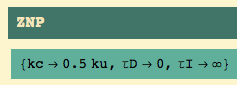
What about the integrated error? We integrate from 0 to t, using as the variable of integration:

(The only difference in those two expressions, I think, is that +0.i disappeared as a result of the Chop command.)

As t goes to infinity, the integrated error tends to a constant positive value:

Now, what does the I-term do in the controller? In the time domain, the controller is

i.e. the I-term is… and tends to 1 as time tends to infinity…

Despite all the terms, the key is the two constants at the beginning:

That’s why the control effort tends to 4. whatever.

Two examples without offset

First, forget that we have PI-control on that plant… imagine that we have our latest closed-loop transfer function, and that it represents an uncontrolled system. What is the G that leads to such a closed-loop transfer function?

That is, we find G such that G / (1+G) = y:

Note that G1 has a pole of order 1 at the origin (i.e. s in the denominator).

Given the warning message, let me check that answer. Use the given open-loop G1 and compute its closed-loop transfer function… and compare it to the one we started with:

And what we see is that if we had started with a plant G that had a pole at zero, then P-only control would have worked.

It’s an interesting game, and I’m sure I’ll be playing it again: usually, set the closed-loop response and the system G, and find the controller K to get the desired closed-loop.

Let me try something simpler. Let’s just take 1/s for the system, and compute the closed-loop transfer function:

Now get the output and control effort in response to a unit step input:

Interesting. Very interesting: the control effort goes to zero… as the error goes to zero… and we do not have offset.

So. As I said at the beginning:

• With P-only control, we may have offset: the output will not tend to the set point.
• In that case, the use of PI-control will eliminate offset.
• But if our plant (G) has a pole of any order at the origin, then P-only control does not lead to offset.
• In that case, you could imagine that the plant itself includes integral control.

Let me be blunt. It would be wrong to say that P-only control always leads to offset.

We recently introduced an exciting feature that has been in planning for some time: immutable aggregate types. In fact, we have been planning to do this for so long that this feature is the subject of our issue #13 on GitHub, out of more than 2400 total issues so far.

Essentially, this feature drastically reduces the overhead of user-defined types that represent small number-like values, or that wrap a small number of other objects. Consider an RGB pixel type:

immutable Pixel
    r::Uint8
    g::Uint8
    b::Uint8
end

Instances of this type can now be packed efficiently into arrays, using exactly 3 bytes per object. In all other respects, these objects continue to act like normal first-class objects. To see how we might use this, here is a function that converts an RGB image in standard 24-bit framebuffer format to grayscale:

function rgb2gray!(img::Array{Pixel})
    for i=1:length(img)
        p = img[i]
        v = uint8(0.30*p.r + 0.59*p.g + 0.11*p.b)
        img[i] = Pixel(v,v,v)
    end
end

This code will run blazing fast, performing no memory allocation. We have not done thorough benchmarking, but this is in fact likely to be the fastest way to write this function in Julia from now on.

The key to this behavior is the new immutable keyword, which means instances of the type cannot be modified. At first this sounds like a mere restriction — how come I’m not allowed to modify one? — but what it really means is that the object is identified with its contents, rather than its memory address. A mutable object has “behavior”; it changes over time, and there may be many references to the object, all of which can observe those changes. An immutable object, on the other hand, has only a value, and no time-varying behavior. Its location does not matter. It is “just some bits”.

Julia has always had some immutable values, in the form of bits types, which are used to represent fixed-bit-width numbers. It is highly intuitive that numbers are immutable. If x equals 2, you might later change the value of x, but it is understood that the value of 2 itself does not change. The immutable keyword generalizes this idea to structured data types with named fields. Julia variables and containers, including arrays, are all still mutable. While a Pixel object itself can’t change, a new Pixel can be written over an old one within an array, since the array is mutable.

Let’s take a look at the benefits of this feature.

1. The compiler and GC have a lot of freedom to move and copy these objects around. This flexibility can be used to store data more efficiently, for example keeping the real and imaginary parts of a complex number in separate registers, or keeping only one part in a register.

2. Immutable objects are easy to reason about. Some languages, such as C++ and C#, provide “value types”, which have many of the benefits of immutable objects. However, their behavior can be confusing. Consider code like the following:

   item = lookup(collection, index) modify!(item) The question here is whether we have modified the same item that is in the collection, or if we have modified a local copy. In Julia there are only two possibilities: either item is mutable, in which case we modified the one and only copy of it, or it is immutable, in which case modifying it is not allowed.

3. No-overhead data abstractions become possible. It is often useful to define a new type that simply wraps a single value, and modifies its behavior in some way. Our favorite modular integer example type fits this description:

   immutable ModInt{n} <: Integer k::Int ModInt(k) = new(mod(k,n)) end Since a given ModInt doesn’t need to exist at a particular address, it can be passed to functions, stored in arrays, and so on, as efficiently as a single Int, with no wrapping overhead. But, in Julia, the overhead will not always be zero. The ModInt type information will “follow the data around” at compile time to the extent possible, but heap-allocated wrappers will be added as needed at run time. Typically these wrappers will be short-lived; if the final destination of a ModInt is in a ModInt array, for example, the wrapper can be discarded when the value is assigned. But if the value is only used locally inside a function, there will most likely be no wrappers at all.

4. Abstractions are fully enforced. If a custom constructor is written for an immutable type, then all instances will be created by it. Since the constructed objects are never modified, the invariants provided by the constructor cannot be violated. At this time, uninitialized arrays are an exception to this rule. New arrays of “plain data” immutable types have unspecified contents, so it is possible to obtain an invalid value from one. This is usually harmless in practice, since arrays must be initialized anyway, and are often created through functions like zeros that do so.

5. We can automatically type-specialize fields. Since field values at construction time are final, their types are too, so we learn everything about the type of an immutable object when it is constructed.

There are many potential optimizations here, and we have not implemented all of them yet. But having this feature in place provides another lever to help us improve performance over time.

For now though, we at least have a much simpler implementation of complex numbers, and will be able to take advantage of efficient rational matrices and other similar niceties.

Addendum: Under the hood

For purposes of calling C and writing reflective code, it helps to know a bit about how immutable types are implemented. Before this change, we had types AbstractKind, BitsKind, and CompositeKind, for separating which types are abstract, which are represented by immutable bit strings, and which are mutable aggregates. It was sometimes convenient that the type system reflected these differences, but also a bit unwarranted since all these types participate in the same hierarchy and follow the same subtyping rules.

Now, the type landscape is both simpler and more complex. The three Kinds have been merged into a single kind called DataType. The type of every value in Julia is now either a DataType, or else a tuple type (union types still exist, but of course are always abstract). To find out the details of a DataType’s physical representation, you must query its properties. DataTypes have three boolean properties abstract, mutable, and pointerfree, and an integer property size. The CompositeKind properties names and types are still there to describe fields.

The abstract property indicates that the type was declared with the abstract keyword and has no direct instances. mutable indicates, for concrete types, whether instances are mutable. pointerfree means that instances contain “just data” and no references to other Julia values. size gives the size of an instance in bytes.

What used to be BitsKinds are now DataTypes that are immutable, concrete, have no fields, and have non-zero size. The former CompositeKinds are mutable and concrete, and either have fields or are zero size if they have zero fields. Clearly, new combinations are now possible. We have already mentioned immutable types with fields. We could have the equivalent of mutable BitsKinds, but this combination is not exposed in the language, since it is easily emulated using mutable fields. Another new combination is abstract types with fields, which would allow you to declare that all subtypes of some abstract type should have certain fields. That one is definitely useful, and we plan to provide syntax for it.

Typically, the only time you need to worry about these things is when calling native code, when you want to know whether some array or struct has C-compatible data layout. This is handled by the type predicate isbits(T).

We held a two day Julia tutorial at MIT in January 2013, which included 10 sessions. MIT Open Courseware and MIT-X graciously provided support for recording of these lectures, so that the wider Julia community can benefit from these sessions.

Julia Lightning Round (slides)

This session is a rapid introduction to julia, using a number of lightning rounds. It uses a number of short examples to demonstrate syntax and features, and gives a quick feel for the language.

Rationale behind Julia and the Vision (slides)

The rationale and vision behind julia, and its design principles are discussed in this session.

Data Analysis with DataFrames (slides)

DataFrames is one of the most widely used Julia packages. This session is an introduction to data analysis with Julia using DataFrames.

Statistical Models in Julia (slides)

This session demonstrates Julia’s statistics capabilities, which are provided by these packages: Distributions, GLM, and LM.

Fast Fourier Transforms

Julia provides a built-in interface to the FFTW library. This session demonstrates the Julia’s signal processing capabilities, such as FFTs and DCTs. Also see the Hadamard package.

Optimization (slides)

This session focuses largely on using Julia for solving linear programming problems. The algebraic modeling language discussed was later released as JuMP. Benchmarks are shown evaluating the performance of Julia for implementing low-level optimization code. Optimization software in Julia has been grouped under the JuliaOpt project.

Metaprogramming and Macros

Julia is homoiconic: it represents its own code as a data structure of the language itself. Since code is represented by objects that can be created and manipulated from within the language, it is possible for a program to transform and generate its own code. Metaprogramming is described in detail in the Julia manual.

Parallel and Distributed Computing (Lab, Solution)

Parallel and distributed computing have been an integral part of Julia’s capabilities from an early stage. This session describes existing basic capabilities, which can be used as building blocks for higher level parallel libraries.

Networking

Julia provides asynchronous networking I/O using the libuv library. Libuv is a portable networking library created as part of the Node.js project.

Grid of Resistors (Lab, Solution)

The Grid of Resistors is a classic numerical problem to compute the voltages and the effective resistance of a 2n+1 by 2n+2 grid of 1 ohm resistors if a battery is connected to the two center points. As part of this lab, the problem is solved in Julia in a number of different ways such as a vectorized implementation, a devectorized implementation, and using comprehensions, in order to study the performance characteristics of various methods.

This post walks through the parallel computing functionality of Julia to implement an asynchronous parallel version of the classical cutting-plane algorithm for convex (nonsmooth) optimization, demonstrating the complete workflow including running on both Amazon EC2 and a large multicore server. I will quickly review the cutting-plane algorithm and will be focusing primarily on parallel computation patterns, so don’t worry if you’re not familiar with the optimization side of things.

Cutting-plane algorithm

The cutting-plane algorithm is a method for solving the optimization problem

where the functions \( f_i \) are convex but not necessarily differentiable. The absolute value function \( |x| \) and the 1-norm \( ||x|| _ 1 \) are typical examples. Important applications also arise from Lagrangian relaxation. The idea of the algorithm is to approximate the functions \( f_i \) with piecewise linear models \( m_i \) which are built up from information obtained by evaluating \( f_i \) at different points. We iteratively minimize over the models to generate candidate solution points.

We can state the algorithm as

1. Choose starting point \( x \).
2. For \(i = 1,\ldots,n\), evaluate \( f_i(x) \) and update corresponding model \( m_i \).
3. Let the next candidate \( x \) be the minimizer of \( \sum_{i=1}^n m_i(x) \).
4. If not converged, goto step 2.

If it is costly to evaluate \( f_i(x) \), then the algorithm is naturally parallelizable at step 2. The minimization in step 3 can be computed by solving a linear optimization problem, which is usually very fast. (Let me point out here that Julia has interfaces to linear programming and other optimization solvers under JuliaOpt.)

Abstracting the math, we can write the algorithm using the following Julia code.

# functions initialize, isconverged, solvesubproblem, and process implemented elsewhere
state, subproblems = initialize()
while !isconverged(state)
    results = map(solvesubproblem,subproblems)
    state, subproblems = process(state, results)
end

The function solvesubproblem corresponds to evaluating \( f_i(x) \) for a given \( i \) and \( x \) (the elements of subproblems could be tuples (i,x)). The function process corresponds to minimizing the model in step 3, and it produces a new state and a new set of subproblems to solve.

Note that the algorithm looks much like a map-reduce that would be easy to parallelize using many existing frameworks. Indeed, in Julia we can simply replace map with pmap (parallel map). Let’s consider a twist that makes the parallelism not so straightforward.

Asynchronous variant

Variability in the time taken by the solvesubproblem function can lead to load imbalance and limit parallel efficiency as workers sit idle waiting for new tasks. Such variability arises naturally if solvesubproblem itself requires solving a optimization problem, or if the workers and network are shared, as is often the case with cloud computing.

We can consider a new variant of the cutting-plane algorithm to address this issue. The key point is

• When proportion \(0 < \alpha \le 1 \) of subproblems for a given candidate have been solved, generate a new candidate and corresponding set of subproblems by using whatever information is presently available.

In other words, we generate new tasks to feed to workers without needing to wait for all current tasks to complete, making the algorithm asynchronous. The algorithm remains convergent, although the total number of iterations may increase. For more details, see this paper by Jeff Linderoth and Stephen Wright.

By introducing asynchronicity we can no longer use a nice black-box pmap function and have to dig deeper into the parallel implementation. Fortunately, this is easy to do in Julia.

Parallel implementation in Julia

Julia implements distributed-memory parallelism based on one-sided message passing, where process push work onto others (via remotecall) and the results are retrieved (via fetch) by the process which requires them. Macros such as @spawn and @parallel provide pretty syntax around this low-level functionality. This model of parallelism is very different from the typical SIMD style of MPI. Both approaches are useful in different contexts, and I expect an MPI wrapper for Julia will appear in the future (see also here).

Reading the manual on parallel computing is highly recommended, and I won’t try to reproduce it in this post. Instead, we’ll dig into and extend one of the examples it presents.

The implementation of pmap in Julia is

function pmap(f, lst)
    np = nprocs()  # determine the number of processors available
    n = length(lst)
    results = cell(n)
    i = 1
    # function to produce the next work item from the queue.
    # in this case it's just an index.
    next_idx() = (idx=i; i+=1; idx)
    @sync begin
        for p=1:np
            if p != myid() || np == 1
                @spawnlocal begin
                    while true
                        idx = next_idx()
                        if idx > n
                            break
                        end
                        results[idx] = remotecall_fetch(p, f, lst[idx])
                    end
                end
            end
        end
    end
    results
end

On first sight, this code is not particularly intuitive. The @spawnlocal macro creates a task on the master process (e.g. process 1). Each task feeds work to a corresponding worker; the call remotecall_fetch(p, f, lst[idx]) function calls f on process p and returns the result when finished. Tasks are uninterruptable and only surrender control at specific points such as remotecall_fetch. Tasks cannot directly modify variables from the enclosing scope, but the same effect can be achieved by using the next_idx function to access and mutate i. The task idiom functions in place of using a loop to poll for results from each worker process.

Implementing our asynchronous algorithm is not much more than a modification of the above code:

# given constants n and 0 < alpha <= 1
# functions initialize and solvesubproblem defined elsewhere
np = nprocs()
state, subproblems = initialize()
converged = false
isconverged() = converged
function updatemodel(mysubproblem, result)
    # store result
    ...
    # decide whether to generate new subproblems
    state.numback[mysubproblem.parent] += 1
    if state.numback[mysubproblem.parent] >= alpha*n && !state.didtrigger[mysubproblem.parent]
        state.didtrigger[mysubproblem.parent] = true
        # generate newsubproblems by solving linear optimization problem
        ...
        if ... # convergence test
            converged = true
        else
            append!(subproblems, newsubproblems)
            push!(state.didtrigger, false)
            push!(state.numback, 0)
            # ensure that for s in newsubproblems, s.parent == length(state.numback)
        end
    end
end

@sync begin
    for p=1:np
        if p != myid() || np == 1
            @spawnlocal begin
                while !isconverged()
                    if length(subproblems) == 0
                        # no more subproblems but haven't converged yet
                        yield()
                        continue
                    end
                    mysubproblem = shift!(subproblems) # pop subproblem from queue
                    result = remotecall_fetch(p, solvesubproblem, mysubproblem)
                    updatemodel(mysubproblem, result)
                end
            end
        end
    end
end

where state is an instance of a type defined as

type State
    didtrigger::Vector{Bool}
    numback::Vector{Int}
    ...
end

There is little difference in the structure of the code inside the @sync blocks, and the asynchronous logic is encapsulated in the local updatemodel function which conditionally generates new subproblems. A strength of Julia is that functions like pmap are implemented in Julia itself, so that it is particularly straightforward to make modifications like this.

Running it

Now for the fun part. The complete cutting-plane algorithm (along with additional variants) is implemented in JuliaBenders. The code is specialized for stochastic programming where the cutting-plane algorithm is known as the L-shaped method or Benders decomposition and is used to decompose the solution of large linear optimization problems. Here, solvesubproblem entails solving a relatively small linear optimization problem. Test instances are taken from the previously mentioned paper.

We’ll first run on a large multicore server. The runals.jl (asynchronous L-shaped) file contains the algorithm we’ll use. Its usage is

julia runals.jl [data source] [num subproblems] [async param] [block size]

where [num subproblems] is the \(n\) as above and [async param] is the proportion \(\alpha\). By setting \(\alpha = 1\) we obtain the synchronous algorithm. For the asynchronous version we will take \(\alpha = 0.6\). The [block size] parameter controls how many subproblems are sent to a worker at once (in the previous code, this value was always 1). We will use 4000 subproblems in our experiments.

To run multiple Julia processes on a shared-memory machine, we pass the -p N option to the julia executable, which will start up N system processes. To execute the asynchronous version with 10 workers, we run

julia -p 12 runals.jl Data/storm 4000 0.6 30

Note that we start 12 processes. These are the 10 workers, the master (which distributes tasks), and another process to perform the master’s computations (an additional refinement which was not described above). Results from various runs are presented in the table below.

Table: Results on a shared-memory 8x Xeon E7-8850 server. Workers correspond to individual cores. Speed is the rate of subproblems solved per second. Efficiency is calculated as the percent of ideal parallel speedup obtained. The superlinear scaling observed with 20 workers is likely a system artifact.

There are a few more hoops to jump through in order to run on EC2. First we must build a system image (AMI) with Julia installed. Julia connects to workers over ssh, so I found it useful to put my EC2 ssh key on the AMI and also set StrictHostKeyChecking no in /etc/ssh/ssh_config to disable the authenticity prompt when connecting to new workers. Someone will likely correct me on if this is the right approach.

Assuming we have an AMI in place, we can fire up the instances. I used an m3.xlarge instance for the master and m1.medium instances for the workers. (Note: you can save a lot of money by using the spot market.)

To add remote workers on startup, Julia accepts a file with a list of host names through the --machinefile option. We can generate this easily enough by using the EC2 API Tools (Ubuntu package ec2-api-tools) with the command

ec2-describe-instances | grep running | awk '{ print $5; }' > mfile

On the master instance we can then run

julia --machinefile mfile runatr.jl Data/storm 4000 0.6 30

Results from various runs are presented in the table below.

Table: Results on Amazon EC2. Workers correspond to individual m1.medium instances. The master process is run on an m3.xlarge instance.

On both architectures the asynchronous version solves subproblems at a higher rate and has significantly better parallel efficiency. Scaling is better on EC2 than on the shared-memory server likely because the subproblem calculation is memory bound, and so performance is better on the distributed-memory architecture. Anyway, with Julia we can easily experiment on both.

Further reading

A more detailed tutorial was prepared for the Julia IAP session at MIT in January 2013.

Distributed Numerical Optimization by Miles Lubin is licensed under a Creative Commons Attribution 4.0 International License.

In a previous article, I followed the various incarnations an instruction takes when it’s being compiled from the source language to machine code in LLVM. The article briefly mentioned a lot of layers within LLVM, each of which is interesting and non trivial.

Here I want to focus on one of the most important and complex layers – the code generator, and specifically the instruction selection mechanism. A short reminder: the task of the code generator is to transform the high-level, mostly target-independent LLVM IR into low-level, target dependent machine language. Instruction selection is the process wherein the abstract operations in IR are mapped to concrete instructions of the target architecture.

This article will follow a simple example to show the instruction selection mechanism in action (ISel in LLVM parlance).

define i64 @imul(i64 %a, i64 %b) nounwind readnone {
entry:
  %mul = mul nsw i64 %b, %a
  ret i64 %mul
}

long imul(long a, long b) {
    return a * b;
}

def IMUL64rr : RI<0xAF, MRMSrcReg, (outs GR64:$dst),
                                   (ins GR64:$src1, GR64:$src2),
                  "imul{q}\t{$src2, $dst|$dst, $src2}",
                  [(set GR64:$dst, EFLAGS,
                        (X86smul_flag GR64:$src1, GR64:$src2))],
                  IIC_IMUL64_RR>,
                 TB;

$ llvm-tblgen lib/Target/X86/X86.td -I=include -I=lib/Target/X86

[(set GR64:$dst, EFLAGS,
      (X86smul_flag GR64:$src1, GR64:$src2))],

def : Pat<(mul GR64:$src1, GR64:$src2),
          (IMUL64rr GR64:$src1, GR64:$src2)>;

// Selection DAG Pattern Support.
//
// Patterns are what are actually matched against by the target-flavored
// instruction selection DAG.  Instructions defined by the target implicitly
// define patterns in most cases, but patterns can also be explicitly added when
// an operation is defined by a sequence of instructions (e.g. loading a large
// immediate value on RISC targets that do not support immediates as large as
// their GPRs).
//

class Pattern<dag patternToMatch, list<dag> resultInstrs> {
  dag             PatternToMatch  = patternToMatch;
  list<dag>       ResultInstrs    = resultInstrs;
  list<Predicate> Predicates      = [];  // See class Instruction in Target.td.
  int             AddedComplexity = 0;   // See class Instruction in Target.td.
}

// Pat - A simple (but common) form of a pattern, which produces a simple result
// not needing a full list.
class Pat<dag pattern, dag result> : Pattern<pattern, [result]>;

Selecting: 0x38c4ee0: i64 = mul 0x38c4de0, 0x38c4be0 [ORD=1] [ID=7]

ISEL: Starting pattern match on root node: 0x38c4ee0: i64 = mul 0x38c4de0, 0x38c4be0 [ORD=1] [ID=7]

  Initial Opcode index to 57917
  Match failed at index 57922
  Continuing at 58133
  Match failed at index 58137
  Continuing at 58246
  Match failed at index 58249
  Continuing at 58335
  TypeSwitch[i64] from 58337 to 58380
MatchAddress: X86ISelAddressMode 0x7fff447ca040
Base_Reg nul Base.FrameIndex 0
 Scale1
IndexReg nul Disp 0
GV nul CP nul
ES nul JT-1 Align0
  Match failed at index 58380
  Continuing at 58396
  Match failed at index 58407
  Continuing at 58516
  Match failed at index 58517
  Continuing at 58531
  Match failed at index 58532
  Continuing at 58544
  Match failed at index 58545
  Continuing at 58557
  Morphed node: 0x38c4ee0: i64,i32 = IMUL64rr 0x38c4de0, 0x38c4be0 [ORD=1]

ISEL: Match complete!
=> 0x38c4ee0: i64,i32 = IMUL64rr 0x38c4de0, 0x38c4be0 [ORD=1]

// The main instruction selector code.
SDNode *SelectCode(SDNode *N) {
  // Some target values are emitted as 2 bytes, TARGET_VAL handles
  // this.
  #define TARGET_VAL(X) X & 255, unsigned(X) >> 8
  static const unsigned char MatcherTable[] = {
/*0*/     OPC_SwitchOpcode /*221 cases */, 73|128,103/*13257*/,  TARGET_VAL(ISD::STORE),// ->13262
/*5*/       OPC_RecordMemRef,
/*6*/       OPC_RecordNode,   // #0 = 'st' chained node
/*7*/       OPC_Scope, 5|128,2/*261*/, /*->271*/ // 7 children in Scope

          /*SwitchOpcode*/ 53|128,8/*1077*/,  TARGET_VAL(ISD::MUL),// ->58994
/*57917*/   OPC_Scope, 85|128,1/*213*/, /*->58133*/ // 7 children in Scope

Initial Opcode index to 57917
Match failed at index 57922
Continuing at 58133

/*58337*/     OPC_SwitchType /*2 cases */, 38,  MVT::i32,// ->58378
/*58340*/       OPC_Scope, 17, /*->58359*/ // 2 children in Scope
/*58342*/         OPC_CheckPatternPredicate, 4, // (!Subtarget->is64Bit())
/*58344*/         OPC_CheckComplexPat, /*CP*/3, /*#*/0, // SelectLEAAddr:$src #1 #2 #3 #4 #5
/*58347*/         OPC_MorphNodeTo, TARGET_VAL(X86::LEA32r), 0,
                      1/*#VTs*/, MVT::i32, 5/*#Ops*/, 1, 2, 3, 4, 5,
                  // Src: lea32addr:i32:$src - Complexity = 18
                  // Dst: (LEA32r:i32 lea32addr:i32:$src)

/*58557*/       /*Scope*/ 12, /*->58570*/
/*58558*/         OPC_CheckType, MVT::i64,
/*58560*/         OPC_MorphNodeTo, TARGET_VAL(X86::IMUL64rr), 0,
                      2/*#VTs*/, MVT::i64, MVT::i32, 2/*#Ops*/, 0, 1,
                  // Src: (mul:i64 GR64:i64:$src1, GR64:i64:$src2) - Complexity = 3
                  // Dst: (IMUL64rr:i64:i32 GR64:i64:$src1, GR64:i64:$src2)

imul:                                   # @imul
      imulq   %rsi, %rdi
      movq    %rdi, %rax
      ret

Conclusion

This article provided an in-depth peek into the instruction selection process – a key part of the LLVM code generator. While it uses a relatively simple example, it should contain sufficient information to gain some initial understanding of the mechanisms involved. In the next part of the article, I will examine a couple of additional examples through which other aspects of the code generation process should become clearer.

[1]	Although the status flags are "implicit" on x86 (there’s no explicit register you can work with), LLVM treats it as explicit to aid the code generation algorithms.

[2]	X86ISD::SMUL is the X86-specific lowering of the generic ISD::SMULO node.

[3]

You may have a "oh my, why is this so complex?" reaction at this point. The TL;DR; answer is "compilers are hard, let’s go fishing". A longer rationale would be: the x86 instruction set is very large and complex. Moreover, LLVM is a compiler with many (quite different) targets and much of its machinery is thus engineered to be target-independent. The result is inherent complexity. To put it differently – the x86 TableGen definitions are about 20 KLOC in size. Add to that another 20 KLOC or so of custom C++ lowering code and compare to the Intel architecture manual which contains 3,000 pages or so. In terms of Kolmogorov complexity, this isn’t very bad

[4]	It’s generated into <BUILD_DIR>/lib/Target/X86/X86GenDAGISel.inc, a file that’s #included by lib/Target/X86/X86ISelDAGToDAG.cpp.

[5]	If you want to understand how this bytecode is generated from the TableGen pattern definitions, you also need to look inside the TableGen DAG ISel backend.

[6]	Note that the values in this table are relevant to the version of LLVM I have built for this example (r174056). Changes in X86 pattern definitions may result in different numbering, but the principle is the same.

[7]	Some multiplications can be optimized to use the faster LEA instruction.

In a previous post, I demonstrated how to use libffi to perform fully dynamic calls to C code, where "fully dynamic" means that even the types of the arguments and return values are determined at runtime.

Here I want to discuss how the same task is done from Python, both with the existing stdlib ctypes package and the new cffi library, developed by the PyPy team and a candidate for inclusion into the Python stdlib in the future.

from ctypes import cdll, Structure, c_int, c_double, c_uint

lib = cdll.LoadLibrary('./libsomelib.so')
print('Loaded lib {0}'.format(lib))

# Describe the DataPoint structure to ctypes.
class DataPoint(Structure):
    _fields_ = [('num', c_int),
                ('dnum', c_double)]

# Initialize the DataPoint[4] argument. Since we just use the DataPoint[4]
# type once, an anonymous instance will do.
dps = (DataPoint * 4)((2, 2.2), (3, 3.3), (4, 4.4), (5, 5.5))

# Grab add_data from the library and specify its return type.
# Note: .argtypes can also be specified
add_data_fn = lib.add_data
add_data_fn.restype = DataPoint

print('Calling add_data via ctypes')
dout = add_data_fn(dps, 4)
print('dout = {0}, {1}'.format(dout.num, dout.dnum))

from cffi import FFI

ffi = FFI()

lib = ffi.dlopen('./libsomelib.so')
print('Loaded lib {0}'.format(lib))

# Describe the data type and function prototype to cffi.
ffi.cdef('''
typedef struct {
    int num;
    double dnum;
} DataPoint;

DataPoint add_data(const DataPoint* dps, unsigned n);
''')

# Create an array of DataPoint structs and initialize it.
dps = ffi.new('DataPoint[]', [(2, 2.2), (3, 3.3), (4, 4.4), (5, 5.5)])

print('Calling add_data via cffi')
# Interesting variation: passing invalid arguments to add_data will trigger
# a cffi type-checking exception.
dout = lib.add_data(dps, 4)
print('dout = {0}, {1}'.format(dout.num, dout.dnum))

from ctypes import (CDLL, byref, Structure, POINTER, c_int,
                    c_void_p, c_long, c_ushort, c_ubyte,
                    c_char, c_char_p, c_void_p)

# CDLL(None) invokes dlopen(NULL), which loads the currently running
# process - in our case Python itself. Since Python is linked with
# libc, readdir_r will be found there.
# Alternatively, we can just explicitly load 'libc.so.6'.
lib = CDLL(None)
print('Loaded lib {0}'.format(lib))

# Describe the types needed for readdir_r.
class DIRENT(Structure):
    _fields_ = [('d_ino', c_long),
                ('d_off', c_long),
                ('d_reclen', c_ushort),
                ('d_type', c_ubyte),
                ('d_name', c_char * 256)]

DIR_p = c_void_p
DIRENT_p = POINTER(DIRENT)
DIRENT_pp = POINTER(DIRENT_p)

# Load the functions we need from the C library. Specify their
# argument and return types.
readdir_r = lib.readdir_r
readdir_r.argtypes = [DIR_p, DIRENT_p, DIRENT_pp]
readdir_r.restype = c_int

opendir = lib.opendir
opendir.argtypes = [c_char_p]
opendir.restype = DIR_p

closedir = lib.closedir
closedir.argtypes = [DIR_p]
closedir.restype = c_int

# opendir's path argument is char*, hence bytes.
path = b'/tmp'
dir_fd = opendir(path)
if not dir_fd:
    raise RuntimeError('opendir failed')

dirent = DIRENT()
result = DIRENT_p()

while True:
    # Note that byref() here is optional since ctypes can do it on its
    # own by observing the argtypes declared for readdir_r. I keep byref
    # for explicitness.
    if readdir_r(dir_fd, byref(dirent), byref(result)):
        raise RuntimeError('readdir_r failed')
    if not result:
        # If (*result == NULL), we're done.
        break
    # dirent.d_name is char[], hence we decode it to get a unicode
    # string.
    print('Found: ' + dirent.d_name.decode('utf-8'))

closedir(dir_fd)

from cffi import FFI

ffi = FFI()
ffi.cdef("""
    typedef void DIR;
    typedef long ino_t;
    typedef long off_t;

    struct dirent {
        ino_t          d_ino;       /* inode number */
        off_t          d_off;       /* offset to the next dirent */
        unsigned short d_reclen;    /* length of this record */
        unsigned char  d_type;      /* type of file; not supported
                                       by all file system types */
        char           d_name[256]; /* filename */
    };

    DIR *opendir(const char *name);
    int readdir_r(DIR *dirp, struct dirent *entry, struct dirent **result);
    int closedir(DIR *dirp);
""")

# Load symbols from the current process (Python).
lib = ffi.dlopen(None)
print('Loaded lib {0}'.format(lib))

path = b'/tmp'
dir_fd = lib.opendir(path)
if not dir_fd:
    raise RuntimeError('opendir failed')

# Allocate the pointers passed to readdir_r.
dirent = ffi.new('struct dirent*')
result = ffi.new('struct dirent**')

while True:
    if lib.readdir_r(dir_fd, dirent, result):
        raise RuntimeError('readdir_r failed')
    if result[0] == ffi.NULL:
        # If (*result == NULL), we're done.
        break
    print('Found: ' + ffi.string(dirent.d_name).decode('utf-8'))

lib.closedir(dir_fd)

A common question is which side of Kullback-Leibler (KL) should I consider for optimization. Since KL is the relative entropy: it is the difference of cross-entropy minus the entropy. As such the ideal model should be on right hand side, and the estimated model on left-hand side. Now suppose you want to find the center of two distributions for mixture simplification. You can interpret the results of left-sided and right-sided KL centroids as follows:

• The Kullback-Leibler right-sided centroid is zero-avoiding so that its corresponding density function tries to cover the support of all input normals,
• The Kullback-Leibler left-sided centroid is zero-forcing so that it focuses on the highest mass mode normal.

Here, there is not one model but two ideal models so we need a trade-off (=centroid). The zero-forcing/avoiding property is depicted in the following figure:

Here are the details (paper).