What is free will? Do we have it? These are difficult questions. Neuroscience seems to point in the direction of determinism. But Christian List suggests that there might still be room for genuine free will.
Tom Rochevery unconvincing
What is free will? Do we have it? These are difficult questions. Neuroscience seems to point in the direction of determinism. But Christian List suggests that there might still be room for genuine free will.
Tom Rocheexcellent historiography and larger themes
Hosted on Acast. See acast.com/privacy for more information.
Tom Rocheboth segments inferior to vast majority of BTN shows
Colleen Eren, author of Bernie Madoff and the Crisis, on why the Ponzi schemer deserves release from prison (op-ed here). Then, Jamieson Webster psychoanalyzes money and left melancholy (interview with Fiona Alison Duncan here).
Tom Rocheexcellent
From its inception as agriculture trade paper in 1843 to the present day, The Economist has provided a gateway into the mind of the banking class. Something of an anomaly in the publishing industry, The Economist is not quite a magazine, not quite a newspaper; aspirational in its branding but bleakly limited in political ambitions; brazenly transparent in its capitalist ideology, yet inscrutable in its favorably spinning for American and British imperialism and racism.
It is publication owned by the wealthy for the wealthy and advertises itself as such. Its only moral pretense: a long history of championing what it calls “liberalism, ”a notoriously slippery term that, in The Economist’s world, views freedom to profit and exploit labor as interchangeable with the freedom of religion, press and speech.
As such, examining The Economist’s history, its connection to British and American banking interests and intelligence services, can tell us a great deal about the narrow focus of Western, and specifically British notions of “liberalism.” The promotion of capital flows over justice, enlightened imperialism over self-determination, abhors overt racism while promoting more subtle forms of race science and colonialism, all along easing the conscience of wealthy white readers that want to feign concern about human suffering but who have everything to gain by doing absolutely nothing about it.
On this episode, we are joined by Alexander Zevin, author of Liberalism at Large: The World According to The Economist.
Tom RocheFebruary 20, 2020 [Colleen Eren @ William Paterson U](https://www.wpunj.edu/cohss/departments/sociology/faculty/colleen-eren.htm), author of [Bernie Madoff and the Crisis](https://www.sup.org/books/title/?id=25123), on why the Ponzi schemer deserves release from prison (op-ed [here](https://www.nytimes.com/2020/02/17/opinion/bernie-madoff-release.html)) • Jamieson Webster psychoanalyzes money and left melancholy (interview with Fiona Alison Duncan [here](https://www.thewhitereview.org/feature/interview-jamieson-webster/))
Tom Rocheaudio @ https://talkpython.fm/episodes/download/252/what-scientific-computing-can-learn-from-cs.mp3
Tom RocheMP3 @ https://traffic.libsyn.com/revolutionspodcast/10.24-_The_Union_of_Struggle_Master.mp3
Relationship Status: Lenin, Plekhanov, and Martov are all on the same side. This won't always be the case.
Sponsor: casper.com/revolutions
Tom Rochecouple great Andrew Maxwell rants oddly deleted from the broadcast version
Tom Rochemore than usually excellent, esp on journeys of the Polos (esp Marco) and of the less wellknown but more astonishing Rabban Bar Ṣawma
Khubilai Khan is a man astride multiple worlds - trying to be both the Khan of the Great Mongol Nation, and the Emperor of the Yuan Dynasty. This will take quite a bit of accommodation, and between Mongolian shamanism, Chinese Confucianism, Buddhism, Daoism, Islam, and Christianity... more than a little behaving like a cultural chameleon to square those civilizational circles.
Learn more about your ad choices. Visit megaphone.fm/adchoices
Tom Roche[Sofia Japaridze @ Solidarity Network Workers Center](https://www.opendemocracy.net/en/odr/investor-standoff-georgia-brings-workers-us-congressmen-conflict/) on Congressionally protected wage theft in the libertarian paradise of post-Soviet Georgia • [Margaret Kimberley @ Black Agenda Report](https://twitter.com/freedomrideblog?lang=en), author of [Prejudential](http://steerforth.com/titles/prejudential/), on the long, oppressive relationship of presidents to black people
Tom Rocheexcellent
Tom Rochevery excellent
Tom Roche[Jessica Whyte @ UNSW](https://www.arts.unsw.edu.au/our-people/jessica-whyte), author of [The Morals of the Market](https://www.versobooks.com/books/3087-the-morals-of-the-market), on the relations between neoliberalism and human rights politics • [Michele Masucci @ Konstfack](https://www.konstfack.se/sv/Aktuellt/Kalender/2018/Red-Love/) and [Joanna Warsza](http://creativetime.org/summit/author/joanna-warsza/), editors of [Red Love](https://mitpress.mit.edu/books/red-love), on Alexandra Kollontai (1872-1952) and her views on love, comradeship, and the family
Note: the 1st/Whyte segment is especially excellent
Tom RocheJohn Clegg @ U Chicago, co-author of [this article](https://catalyst-journal.com/vol3/no3/the-economic-origins-of-mass-incarceration), on the economic roots of mass incarceration • Tobita Chow @ Justice Is Global & Jake Werner @ U Chicago, authors of [this paper](http://www.rosalux-nyc.org/the-us-china-trade-war/), on the US–China trade war
Tom Rocheexcellent pullquotes:
> with fewer workers per retiree, it will be harder to support retirement programs. The problem with the story is that the benefits from higher productivity growth swamp any possible increase in costs associated with changes in demographics. Here is what I [wrote](http://cepr.net/blogs/beat-the-press/more-nonsense-on-china-s-demography) a few years back in reference to China.
> > Suppose that China starts out with five workers per retiree, each with a wage before payments for retirees of 100. Let's assume that the living standard of retirees requires that them to have 80 percent of the income of an average worker. In this story, we would need a tax rate of 13.8 percentage points on wages to maintain this living standard for retirees. This makes the wage net of payments to support the retired population equal to 86.2.
> > Now suppose that over two decades the population ages so that the ratio of workers to retirees is just two to one. However, suppose over this two decade period productivity growth (output per worker hour) averages 5.0 percent annually. If we first calculate the tax rate needed to maintain a living standard for retirees, it is now 28.6 percent, leaving our worker with 71.4 percent of their pre-tax wage.
> > But as a result of 5.0 percent annual productivity growth, the before tax wage will 265.3 percent of its level from twenty years earlier. This means that the pay net of the tax to support retirees would be 189.3 percent of the average before tax wage from twenty years earlier. If we compare after-tax wages for the two periods, the after-tax wage in the second period would be 219.6 percent of the after-tax wage in the first period. The living standards of retirees would also be correspondingly higher.
...
> While a 5 percent annual rate of productivity growth is plausible for China, it is certainly too high for the U.S., Europe and Japan. A more reasonable rate would be 1.0-1.5 percent. (Sorry, there is no evidence in these data that the robots are coming.) But even taking a 1.0 percent rate of productivity growth, the before tax wage (assuming wages keep pace with productivity growth) will be 22 percent higher in two decades. That is far more than enough to offset any tax increases needed to support plausible increases in the ratio of retirees to workers. [... The] problem is intra-generational inequality, not inter-generational inequality.
> Finally, we have the story that in a country like Japan, a declining population might mean that it cannot sustain economic growth. The proper response here is, who cares? Insofar as we are interested in growth at all, we care about per capita growth. If Japan's population declines 1.0 percent a year and its economy shrinks modestly (say 0.2-0.3 percent annually), this is still consistent with a rise in per capita GDP of 0.7-0.8 percent annually. That's not super-fast, but still decent for a wealthy country. And, if Japan chooses to take the benefits of higher productivity in the form of shorter work weeks and work years, as it has done over the last three decades, why is this is a problem?
Folks who have followed economic policy debates for the last few decades can never be surprised by the poor quality of reporting, but it still can get annoying. In a world where we are already doing irreparable damage to the environment through global warming, the idea that we will have fewer people in the future should be seen as a good thing.
Nonetheless, our leading news outlets are warning us that China, the world's most heavily populated country may be seeing its population decline in the decades ahead. The story is that fewer babies will mean fewer workers twenty years out. We are warned that this would lead to a labor shortage and make it more difficult to support retirement pensions. The Post article warns that in Japan (it also talks about countries other than China), it could make it difficult to sustain economic growth.
Let's deal with these one by one. What does a labor shortage mean? Presumably it will be hard to get people to do the least productive, lowest paying jobs. The obvious response is, so what? This is called "capitalism." If a particular job holds little value then it won't get done. This is the reason half of our workforce is not still in agriculture. They are doing more productive tasks elsewhere.
Going forward, if we do see serious labor shortages we will probably see fewer people serving tables in restaurants, working as housekeepers in hotels or providing valet parking. And, the people who still work at these jobs will get much higher pay. Sounds like a terrible crisis!
The second point is that with fewer workers per retiree, it will be harder to support retirement programs. The problem with the story is that the benefits from higher productivity growth swamp any possible increase in costs associated with changes in demographics. Here is what I wrote a few years back in reference to China.
Tom Rocheexcellent survey of more-complicated-than-usually-taught history
Stephen Tomkins discusses the rise of Puritanism in England and the origins of the Mayflower voyage to North America in 1620. Historyextra.com/podcast
See acast.com/privacy for privacy and opt-out information.
Tom Roche[James Meadway](https://www.ippr.org/about/people/staff/james-meadway), former economic advisor to the UK Labour Party, on the British election, how to fight political cynicism, and [ideas](https://tribunemag.co.uk/2019/07/dedeindustrialisation) for reindustrializing busted regions • [Katherine Moos](http://www.katherinemoos.com/) on the costs of social reproduction and who pays them (paper [here](https://www.tandfonline.com/doi/abs/10.1080/00346764.2019.1703031?scroll=top&journalCode=rrse20))
Tom Rochemuch funnier than the broadcast
Tom Rochethe Schrader piece is excellent
Writer Jeff Sparrow on the Australian fires. Then, Stuart Schrader, author of Badges Without Borders, on counterinsurgency and policing.
Tom Rochebetter content (not audio) link: https://www.npr.org/2020/01/08/794509417/american-oligarchs-reveals-how-trump-kushner-families-learned-to-work-the-system
Tom Rochegetting 403 @ 2020 UTC F 10 Jan 2020. retried, complained via https://www.bbc.co.uk/contact/complaints/make-a-complaint/ @ 1400 (2100 UTC)
Tom RocheShahin Khan does good quick intro to quantum computing in the 'Things You Think You Know' segment (10:58-14:12), plus the linked-to (in the text for this episode) Saturday Morning Breakfast Cereal comic @ http://www.smbc-comics.com/comic/the-talk-3 (archived @ https://web.archive.org/web/20200103193819/http://www.smbc-comics.com/comic/the-talk-3 ) is also very much worth the few minutes read.

Tom Rochevery important basics
Do you have a large dataset that’s full of interesting insights, but you’re not sure where to start exploring it? Has your boss asked you to generate some statistics from it, but they’re not so easy to extract? These are precisely the use cases where Pandas and Python can help you! With these tools, you’ll be able to slice a large dataset down into manageable parts and glean insight from that information.
In this tutorial, you’ll learn how to:
You’ll also learn about the differences between the main data structures that Pandas and Python use. To follow along, you can get all of the example code in this tutorial at the link below:
Get Jupyter Notebook: Click here get the Jupyter Notebook you'll use to explore data with Pandas in this tutorial.
There are a few things you’ll need to get started with this tutorial. First is a familiarity with Python’s built-in data structures, especially lists and dictionaries. For more information, check out Lists and Tuples in Python and Dictionaries in Python.
The second thing you’ll need is a working Python environment. You can follow along in any terminal that has Python 3 installed. If you want to see nicer output, especially for the large NBA dataset you’ll be working with, then you might want to run the examples in a Jupyter notebook.
Note: If you don’t have Python installed at all, then check out Python 3 Installation & Setup Guide. You can also follow along online in a try-out Jupyter notebook.
The last thing you’ll need is the Pandas Python library, which you can install with pip:
$ python -m pip install pandas
You can also use the Conda package manager:
$ conda install pandas
If you’re using the Anaconda distribution, then you’re good to go! Anaconda already comes with the Pandas Python library installed.
Note: Have you heard that there are multiple package managers in the Python world and are somewhat confused about which one to pick? pip and conda are both excellent choices, and they each have their advantages.
If you’re going to use Python mainly for data science work, then conda is perhaps the better choice. In the conda ecosystem, you have two main alternatives:
The examples in this tutorial have been tested with Python 3.7 and Pandas 0.25.0, but they should also work in older versions. You can get all the code examples you’ll see in this tutorial in a Jupyter notebook by clicking the link below:
Get Jupyter Notebook: Click here get the Jupyter Notebook you'll use to explore data with Pandas in this tutorial.
Let’s get started!
Now that you’ve installed Pandas, it’s time to have a look at a dataset. In this tutorial, you’ll analyze NBA results provided by FiveThirtyEight in a 17MB CSV file. Create a script download_nba_all_elo.py to download the data:
import requests

download_url = "https://raw.githubusercontent.com/fivethirtyeight/data/master/nba-elo/nbaallelo.csv"
target_csv_path = "nba_all_elo.csv"

response = requests.get(download_url)
response.raise_for_status()    # Check that the request was successful
with open(target_csv_path, "wb") as f:
    f.write(response.content)
print("Download ready.")
When you execute the script, it will save the file nba_all_elo.csv in your current working directory.
Note: You could also use your web browser to download the CSV file.
However, having a download script has several advantages:
Now you can use the Pandas Python library to take a look at your data:
>>> import pandas as pd
>>> nba = pd.read_csv("nba_all_elo.csv")
>>> type(nba)
<class 'pandas.core.frame.DataFrame'>
Here, you follow the convention of importing Pandas in Python with the pd alias. Then, you use .read_csv() to read in your dataset and store it as a DataFrame object in the variable nba.
Note: Is your data not in CSV format? No worries! The Pandas Python library provides several similar functions like read_json(), read_html(), and read_sql_table(). To learn how to work with these file formats, check out Reading and Writing Files With Pandas or consult the docs.
You can see how much data nba contains:
>>> len(nba)
126314
>>> nba.shape
(126314, 23)
You use the Python built-in function len() to determine the number of rows. You also use the .shape attribute of the DataFrame to see its dimensionality. The result is a tuple containing the number of rows and columns.
Now you know that there are 126,314 rows and 23 columns in your dataset. But how can you be sure the dataset really contains basketball stats? You can have a look at the first five rows with .head():
>>> nba.head()
If you’re following along with a Jupyter notebook, then you’ll see a result like this:
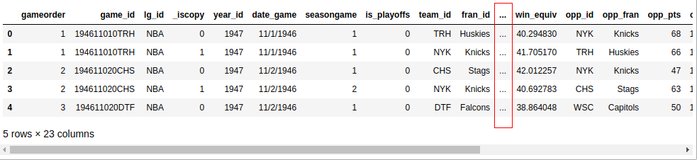
Unless your screen is quite large, your output probably won’t display all 23 columns. Somewhere in the middle, you’ll see a column of ellipses (...) indicating the missing data. If you’re working in a terminal, then that’s probably more readable than wrapping long rows. However, Jupyter notebooks will allow you to scroll. You can configure Pandas to display all 23 columns like this:
>>> pd.set_option("display.max.columns", None)
While it’s practical to see all the columns, you probably won’t need six decimal places! Change it to two:
>>> pd.set_option("display.precision", 2)
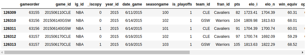
To verify that you’ve changed the options successfully, you can execute .head() again, or you can display the last five rows with .tail() instead:
>>> nba.tail()
Now, you should see all the columns, and your data should show two decimal places:
You can discover some further possibilities of .head() and .tail() with a small exercise. Can you print the last three lines of your DataFrame? Expand the code block below to see the solution:
Solution: head & tail Show/Hide
Here’s how to print the last three lines of nba:
>>> nba.tail(3)
Your output should look something like this:
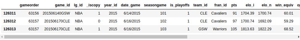
You can see the last three lines of your dataset with the options you’ve set above.
Similar to the Python standard library, functions in Pandas also come with several optional parameters. Whenever you bump into an example that looks relevant but is slightly different from your use case, check out the official documentation. The chances are good that you’ll find a solution by tweaking some optional parameters!
You’ve imported a CSV file with the Pandas Python library and had a first look at the contents of your dataset. So far, you’ve only seen the size of your dataset and its first and last few rows. Next, you’ll learn how to examine your data more systematically.
The first step in getting to know your data is to discover the different data types it contains. While you can put anything into a list, the columns of a DataFrame contain values of a specific data type. When you compare Pandas and Python data structures, you’ll see that this behavior makes Pandas much faster!
You can display all columns and their data types with .info():
>>> nba.info()
This will produce the following output:
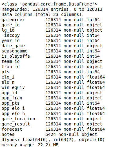
You’ll see a list of all the columns in your dataset and the type of data each column contains. Here, you can see the data types int64, float64, and object. Pandas uses the NumPy library to work with these types. Later, you’ll meet the more complex categorical data type, which the Pandas Python library implements itself.
The object data type is a special one. According to the Pandas Cookbook, the object data type is “a catch-all for columns that Pandas doesn’t recognize as any other specific type.” In practice, it often means that all of the values in the column are strings.
Although you can store arbitrary Python objects in the object data type, you should be aware of the drawbacks to doing so. Strange values in an object column can harm Pandas’ performance and its interoperability with other libraries. For more information, check out the official getting started guide.
Now that you’ve seen what data types are in your dataset, it’s time to get an overview of the values each column contains. You can do this with .describe():
>>> nba.describe()
This function shows you some basic descriptive statistics for all numeric columns:
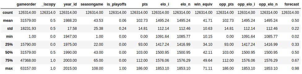
.describe() only analyzes numeric columns by default, but you can provide other data types if you use the include parameter:
>>> import numpy as np
>>> nba.describe(include=np.object)
.describe() won’t try to calculate a mean or a standard deviation for the object columns, since they mostly include text strings. However, it will still display some descriptive statistics:
Take a look at the team_id and fran_id columns. Your dataset contains 104 different team IDs, but only 53 different franchise IDs. Furthermore, the most frequent team ID is BOS, but the most frequent franchise ID Lakers. How is that possible? You’ll need to explore your dataset a bit more to answer this question.
Exploratory data analysis can help you answer questions about your dataset. For example, you can examine how often specific values occur in a column:
>>> nba["team_id"].value_counts()
BOS    5997
NYK    5769
LAL    5078
...
SDS      11
>>> nba["fran_id"].value_counts()
Name: team_id, Length: 104, dtype: int64
Lakers          6024
Celtics         5997
Knicks          5769
...
Huskies           60
Name: fran_id, dtype: int64
It seems that a team named "Lakers" played 6024 games, but only 5078 of those were played by the Los Angeles Lakers. Find out who the other "Lakers" team is:
>>> nba.loc[nba["fran_id"] == "Lakers", "team_id"].value_counts()
LAL    5078
MNL     946
Name: team_id, dtype: int64
Indeed, the Minneapolis Lakers ("MNL") played 946 games. You can even find out when they played those games:
>>> nba.loc[nba["team_id"] == "MNL", "date_game"].min()
'1/1/1949'
>>> nba.loc[nba["team_id"] == "MNL", "date_game"].max()
'4/9/1959'
>>> nba.loc[nba["team_id"] == "MNL", "date_game"].agg(("min", "max"))
min    1/1/1949
max    4/9/1959
Name: date_game, dtype: object
It looks like the Minneapolis Lakers played between the years of 1949 and 1959. That explains why you might not recognize this team!
You’ve also found out why the Boston Celtics team "BOS" played the most games in the dataset. Let’s analyze their history also a little bit. Find out how many points the Boston Celtics have scored during all matches contained in this dataset. Expand the code block below for the solution:
Solution: DataFrame intro Show/Hide
Similar to the .min() and .max() aggregate functions, you can also use .sum():
>>> nba.loc[nba["team_id"] == "BOS", "pts"].sum()
626484
The Boston Celtics scored a total of 626,484 points.
You’ve got a taste for the capabilities of a Pandas DataFrame. In the following sections, you’ll expand on the techniques you’ve just used, but first, you’ll zoom in and learn how this powerful data structure works.
While a DataFrame provides functions that can feel quite intuitive, the underlying concepts are a bit trickier to understand. For this reason, you’ll set aside the vast NBA DataFrame and build some smaller Pandas objects from scratch.
Python’s most basic data structure is the list, which is also a good starting point for getting to know pandas.Series objects. Create a new Series object based on a list:
>>> revenues = pd.Series([5555, 7000, 1980])
>>> revenues
0    5555
1    7000
2    1980
dtype: int64
You’ve used the list [5555, 7000, 1980] to create a Series object called revenues. A Series object wraps two components:
You can access these components with .values and .index, respectively:
>>> revenues.values
array([5555, 7000, 1980])
>>> revenues.index
RangeIndex(start=0, stop=3, step=1)
revenues.values returns the values in the Series, whereas revenues.index returns the positional index.
Note: If you’re familiar with NumPy, then it might be interesting for you to note that the values of a Series object are actually n-dimensional arrays:
>>> type(revenues.values)
<class 'numpy.ndarray'>
If you’re not familiar with NumPy, then there’s no need to worry! You can explore the ins and outs of your dataset with the Pandas Python library alone. However, if you’re curious about what Pandas does behind the scenes, then check out Look Ma, No For-Loops: Array Programming With NumPy.
While Pandas builds on NumPy, a significant difference is in their indexing. Just like a NumPy array, a Pandas Series also has an integer index that’s implicitly defined. This implicit index indicates the element’s position in the Series.
However, a Series can also have an arbitrary type of index. You can think of this explicit index as labels for a specific row:
>>> city_revenues = pd.Series(
...     [4200, 8000, 6500],
...     index=["Amsterdam", "Toronto", "Tokyo"]
... )
>>> city_revenues
Amsterdam    4200
Toronto      8000
Tokyo        6500
dtype: int64
Here, the index is a list of city names represented by strings. You may have noticed that Python dictionaries use string indices as well, and this is a handy analogy to keep in mind! You can use the code blocks above to distinguish between two types of Series:
revenues: This Series behaves like a Python list because it only has a positional index.city_revenues: This Series acts like a Python dictionary because it features both a positional and a label index.Here’s how to construct a Series with a label index from a Python dictionary:
>>> city_employee_count = pd.Series({"Amsterdam": 5, "Tokyo": 8})
>>> city_employee_count
Amsterdam    5
Tokyo        8
dtype: int64
The dictionary keys become the index, and the dictionary values are the Series values.
Just like dictionaries, Series also support .keys() and the in keyword:
>>> city_employee_count.keys()
Index(['Amsterdam', 'Tokyo'], dtype='object')
>>> "Tokyo" in city_employee_count
True
>>> "New York" in city_employee_count
False
You can use these methods to answer questions about your dataset quickly.
While a Series is a pretty powerful data structure, it has its limitations. For example, you can only store one attribute per key. As you’ve seen with the nba dataset, which features 23 columns, the Pandas Python library has more to offer with its DataFrame. This data structure is a sequence of Series objects that share the same index.
If you’ve followed along with the Series examples, then you should already have two Series objects with cities as keys:
city_revenuescity_employee_countYou can combine these objects into a DataFrame by providing a dictionary in the constructor. The dictionary keys will become the column names, and the values should contain the Series objects:
>>> city_data = pd.DataFrame({
...     "revenue": city_revenues,
...     "employee_count": city_employee_count
... })
>>> city_data
           revenue  employee_count
Amsterdam     4200             5.0
Tokyo         6500             8.0
Toronto       8000             NaN
Note how Pandas replaced the missing employee_count value for Toronto with NaN.
The new DataFrame index is the union of the two Series indices:
>>> city_data.index
Index(['Amsterdam', 'Tokyo', 'Toronto'], dtype='object')
Just like a Series, a DataFrame also stores its values in a NumPy array:
>>> city_data.values
array([[4.2e+03, 5.0e+00],
       [6.5e+03, 8.0e+00],
       [8.0e+03,     nan]])
You can also refer to the 2 dimensions of a DataFrame as axes:
>>> city_data.axes
[Index(['Amsterdam', 'Tokyo', 'Toronto'], dtype='object'),
 Index(['revenue', 'employee_count'], dtype='object')]
>>> city_data.axes[0]
 Index(['Amsterdam', 'Tokyo', 'Toronto'], dtype='object')
>>> city_data.axes[1]
 Index(['revenue', 'employee_count'], dtype='object')
The axis marked with 0 is the row index, and the axis marked with 1 is the column index. This terminology is important to know because you’ll encounter several DataFrame methods that accept an axis parameter.
A DataFrame is also a dictionary-like data structure, so it also supports .keys() and the in keyword. However, for a DataFrame these don’t relate to the index, but to the columns:
>>> city_data.keys()
Index(['revenue', 'employee_count'], dtype='object')
>>> "Amsterdam" in city_data
False
>>> "revenue" in city_data
True
You can see these concepts in action with the bigger NBA dataset. Does it contain a column called "points", or was it called "pts"? To answer this question, display the index and the axes of the nba dataset, then expand the code block below for the solution:
Solution: NBA index Show/Hide
Because you didn’t specify an index column when you read in the CSV file, Pandas has assigned a RangeIndex to the DataFrame:
>>> nba.index
RangeIndex(start=0, stop=126314, step=1)
nba, like all DataFrame objects, has two axes:
>>> nba.axes
[RangeIndex(start=0, stop=126314, step=1),
 Index(['gameorder', 'game_id', 'lg_id', '_iscopy', 'year_id', 'date_game',
        'seasongame', 'is_playoffs', 'team_id', 'fran_id', 'pts', 'elo_i',
        'elo_n', 'win_equiv', 'opp_id', 'opp_fran', 'opp_pts', 'opp_elo_i',
        'opp_elo_n', 'game_location', 'game_result', 'forecast', 'notes'],
       dtype='object')]
You can check the existence of a column with .keys():
>>> "points" in nba.keys()
False
>>> "pts" in nba.keys()
True
The column is called "pts", not "points".
As you use these methods to answer questions about your dataset, be sure to keep in mind whether you’re working with a Series or a DataFrame so that your interpretation is accurate.
In the section above, you’ve created a Pandas Series based on a Python list and compared the two data structures. You’ve seen how a Series object is similar to lists and dictionaries in several ways. A further similarity is that you can use the indexing operator ([]) for Series as well.
You’ll also learn how to use two Pandas-specific access methods:
.loc.ilocYou’ll see that these data access methods can be much more readable than the indexing operator.
Recall that a Series has two indices:
RangeIndex
Next, revisit the city_revenues object:
>>> city_revenues
Amsterdam    4200
Toronto      8000
Tokyo        6500
dtype: int64
You can conveniently access the values in a Series with both the label and positional indices:
>>> city_revenues["Toronto"]
8000
>>> city_revenues[1]
8000
You can also use negative indices and slices, just like you would for a list:
>>> city_revenues[-1]
6500
>>> city_revenues[1:]
Toronto    8000
Tokyo      6500
dtype: int64
>>> city_revenues["Toronto":]
Toronto    8000
Tokyo      6500
dtype: int64
If you want to learn more about the possibilities of the indexing operator, then check out Lists and Tuples in Python.
.loc and .iloc
The indexing operator ([]) is convenient, but there’s a caveat. What if the labels are also numbers? Say you have to work with a Series object like this:
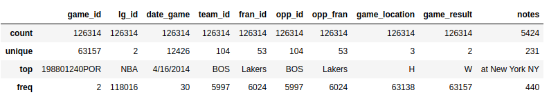
>>> colors = pd.Series(
...     ["red", "purple", "blue", "green", "yellow"],
...     index=[1, 2, 3, 5, 8]
... )
>>> colors
1       red
2    purple
3      blue
5     green
8    yellow
dtype: object
What will colors[1] return? For a positional index, colors[1] is "purple". However, if you go by the label index, then colors[1] is referring to "red".
The good news is, you don’t have to figure it out! Instead, to avoid confusion, the Pandas Python library provides two data access methods:
.loc refers to the label index..iloc refers to the positional index.These data access methods are much more readable:
>>> colors.loc[1]
'red'
>>> colors.iloc[1]
'purple'
colors.loc[1] returned "red", the element with the label 1. colors.iloc[1] returned "purple", the element with the index 1.
The following figure shows which elements .loc and .iloc refer to:
Again, .loc points to the label index on the right-hand side of the image. Meanwhile, .iloc points to the positional index on the left-hand side of the picture.
It’s easier to keep in mind the distinction between .loc and .iloc than it is to figure out what the indexing operator will return. Even if you’re familiar with all the quirks of the indexing operator, it can be dangerous to assume that everybody who reads your code has internalized those rules as well!
Note: In addition to being confusing for Series with numeric labels, the Python indexing operator has some performance drawbacks. It’s perfectly okay to use it in interactive sessions for ad-hoc analysis, but for production code, the .loc and .iloc data access methods are preferable. For further details, check out the Pandas User Guide section on indexing and selecting data.
.loc and .iloc also support the features you would expect from indexing operators, like slicing. However, these data access methods have an important difference. While .iloc excludes the closing element, .loc includes it. Take a look at this code block:
>>> # Return the elements with the implicit index: 1, 2
>>> colors.iloc[1:3]
2    purple
3      blue
dtype: object
If you compare this code with the image above, then you can see that colors.iloc[1:3] returns the elements with the positional indices of 1 and 2. The closing item "green" with a positional index of 3 is excluded.
On the other hand, .loc includes the closing element:
>>> # Return the elements with the explicit index between 3 and 8
>>> colors.loc[3:8]
3      blue
5     green
8    yellow
dtype: object
This code block says to return all elements with a label index between 3 and 8. Here, the closing item "yellow" has a label index of 8 and is included in the output.
You can also pass a negative positional index to .iloc:
>>> colors.iloc[-2]
'green'
You start from the end of the Series and return the second element.
Note: There used to be an .ix indexer, which tried to guess whether it should apply positional or label indexing depending on the data type of the index. Because it caused a lot of confusion, it has been deprecated since Pandas version 0.20.0.
It’s highly recommended that you do not use .ix for indexing. Instead, always use .loc for label indexing and .iloc for positional indexing. For further details, check out the Pandas User Guide.
You can use the code blocks above to distinguish between two Series behaviors:
.iloc on a Series similar to using [] on a list..loc on a Series similar to using [] on a dictionary.Be sure to keep these distinctions in mind as you access elements of your Series objects.
Since a DataFrame consists of Series objects, you can use the very same tools to access its elements. The crucial difference is the additional dimension of the DataFrame. You’ll use the indexing operator for the columns and the access methods .loc and .iloc on the rows.
If you think of a DataFrame as a dictionary whose values are Series, then it makes sense that you can access its columns with the indexing operator:
>>> city_data["revenue"]
Amsterdam    4200
Tokyo        6500
Toronto      8000
Name: revenue, dtype: int64
>>> type(city_data["revenue"])
pandas.core.series.Series
Here, you use the indexing operator to select the column labeled "revenue".
If the column name is a string, then you can use attribute-style accessing with dot notation as well:
>>> city_data.revenue
Amsterdam    4200
Tokyo        6500
Toronto      8000
Name: revenue, dtype: int64
city_data["revenue"] and city_data.revenue return the same output.
There’s one situation where accessing DataFrame elements with dot notation may not work or may lead to surprises. This is when a column name coincides with a DataFrame attribute or method name:
>>> toys = pd.DataFrame([
...     {"name": "ball", "shape": "sphere"},
...     {"name": "Rubik's cube", "shape": "cube"}
... ])
>>> toys["shape"]
0    sphere
1      cube
Name: shape, dtype: object
>>> toys.shape
(2, 2)
The indexing operation toys["shape"] returns the correct data, but the attribute-style operation toys.shape still returns the shape of the DataFrame. You should only use attribute-style accessing in interactive sessions or for read operations. You shouldn’t use it for production code or for manipulating data (such as defining new columns).
.loc and .iloc
Similar to Series, a DataFrame also provides .loc and .iloc data access methods. Remember, .loc uses the label and .iloc the positional index:
>>> city_data.loc["Amsterdam"]
revenue           4200.0
employee_count       5.0
Name: Amsterdam, dtype: float64
>>> city_data.loc["Tokyo": "Toronto"]
        revenue employee_count
Tokyo   6500    8.0
Toronto 8000    NaN
>>> city_data.iloc[1]
revenue           6500.0
employee_count       8.0
Name: Tokyo, dtype: float64
Each line of code selects a different row from city_data:
city_data.loc["Amsterdam"] selects the row with the label index "Amsterdam".city_data.loc["Tokyo": "Toronto"] selects the rows with label indices from "Tokyo" to "Toronto". Remember, .loc is inclusive.city_data.iloc[1] selects the row with the positional index 1, which is "Tokyo".Alright, you’ve used .loc and .iloc on small data structures. Now, it’s time to practice with something bigger! Use a data access method to display the second-to-last row of the nba dataset. Then, expand the code block below to see a solution:
Solution: NBA accessing rows Show/Hide
The second-to-last row is the row with the positional index of -2. You can display it with .iloc:
>>> nba.iloc[-2]
gameorder               63157
game_id          201506170CLE
lg_id                     NBA
_iscopy                     0
year_id                  2015
date_game           6/16/2015
seasongame                102
is_playoffs                 1
team_id                   CLE
fran_id             Cavaliers
pts                        97
elo_i                 1700.74
elo_n                 1692.09
win_equiv             59.2902
opp_id                    GSW
opp_fran             Warriors
opp_pts                   105
opp_elo_i             1813.63
opp_elo_n             1822.29
game_location               H
game_result                 L
forecast              0.48145
notes                     NaN
Name: 126312, dtype: object
You’ll see the output as a Series object.
For a DataFrame, the data access methods .loc and .iloc also accept a second parameter. While the first parameter selects rows based on the indices, the second parameter selects the columns. You can use these parameters together to select a subset of rows and columns from your DataFrame:
>>> city_data.loc["Amsterdam": "Tokyo", "revenue"]
Amsterdam    4200
Tokyo        6500
Name: revenue, dtype: int64
Note that you separate the parameters with a comma (,). The first parameter, "Amsterdam" : "Tokyo," says to select all rows between those two labels. The second parameter comes after the comma and says to select the "revenue" column.
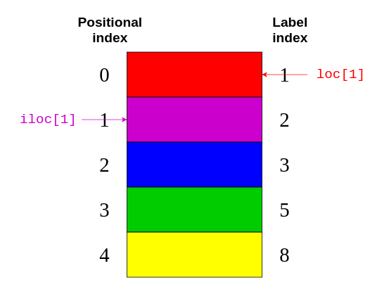
It’s time to see the same construct in action with the bigger nba dataset. Select all games between the labels 5555 and 5559. You’re only interested in the names of the teams and the scores, so select those elements as well. Expand the code block below to see a solution:
Solution: NBA accessing a subset Show/Hide
First, define which rows you want to see, then list the relevant columns:
>>> nba.loc[5555:5559, ["fran_id", "opp_fran", "pts", "opp_pts"]]
You use .loc for the label index and a comma (,) to separate your two parameters.
You should see a small part of your quite huge dataset:
The output is much easier to read!
With data access methods like .loc and .iloc, you can select just the right subset of your DataFrame to help you answer questions about your dataset.
You’ve seen how to access subsets of a huge dataset based on its indices. Now, you’ll select rows based on the values in your dataset’s columns to query your data. For example, you can create a new DataFrame that contains only games played after 2010:
>>> current_decade = nba[nba["year_id"] > 2010]
>>> current_decade.shape
(12658, 23)
You still have all 23 columns, but your new DataFrame only consists of rows where the value in the "year_id" column is greater than 2010.
You can also select the rows where a specific field is not null:
>>> games_with_notes = nba[nba["notes"].notnull()]
>>> games_with_notes.shape
(5424, 23)
This can be helpful if you want to avoid any missing values in a column. You can also use .notna() to achieve the same goal.
You can even access values of the object data type as str and perform string methods on them:
>>> ers = nba[nba["fran_id"].str.endswith("ers")]
>>> ers.shape
(27797, 23)
You use .str.endswith() to filter your dataset and find all games where the home team’s name ends with "ers".
You can combine multiple criteria and query your dataset as well. To do this, be sure to put each one in parentheses and use the logical operators | and & to separate them.
Note: The operators and, or, &&, and || won’t work here. If you’re curious as to why then check out the section on how the Pandas Python library uses Boolean operators in Python Pandas: Tricks & Features You May Not Know.
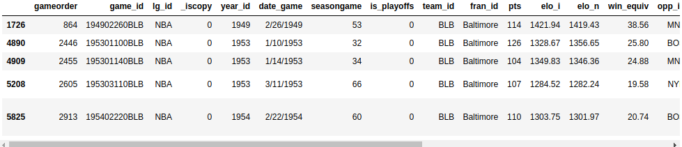
Do a search for Baltimore games where both teams scored over 100 points. In order to see each game only once, you’ll need to exclude duplicates:
>>> nba[
...     (nba["_iscopy"] == 0) &
...     (nba["pts"] > 100) &
...     (nba["opp_pts"] > 100) &
...     (nba["team_id"] == "BLB")
... ]
Here, you use nba["_iscopy"] == 0 to include only the entries that aren’t copies.
Your output should contain five eventful games:
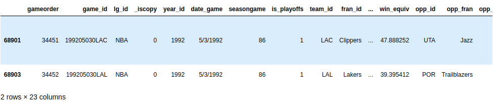
Try to build another query with multiple criteria. In the spring of 1992, both teams from Los Angeles had to play a home game at another court. Query your dataset to find those two games. Both teams have an ID starting with "LA". Expand the code block below to see a solution:
Solution: Queries Show/Hide
You can use .str to find the team IDs that start with "LA", and you can assume that such an unusual game would have some notes:
>>> nba[
...     (nba["_iscopy"] == 0) &
...     (nba["team_id"].str.startswith("LA")) &
...     (nba["year_id"]==1992) &
...     (nba["notes"].notnull())
... ]
Your output should show two games on the day 5/3/1992:
Nice find!
When you know how to query your dataset with multiple criteria, you’ll be able to answer more specific questions about your dataset.
You may also want to learn other features of your dataset, like the sum, mean, or average value of a group of elements. Luckily, the Pandas Python library offers grouping and aggregation functions to help you accomplish this task.
A Series has more than twenty different methods for calculating descriptive statistics. Here are some examples:
>>> city_revenues.sum()
18700
>>> city_revenues.max()
8000
The first method returns the total of city_revenues, while the second returns the max value. There are other methods you can use, like .min() and .mean().
Remember, a column of a DataFrame is actually a Series object. For this reason, you can use these same functions on the columns of nba:
>>> points = nba["pts"]
>>> type(points)
<class 'pandas.core.series.Series'>
>>> points.sum()
12976235
A DataFrame can have multiple columns, which introduces new possibilities for aggregations, like grouping:
>>> nba.groupby("fran_id", sort=False)["pts"].sum()
fran_id
Huskies           3995
Knicks          582497
Stags            20398
Falcons           3797
Capitols         22387
...
By default, Pandas sorts the group keys during the call to .groupby(). If you don’t want to sort, then pass sort=False. This parameter can lead to performance gains.
You can also group by multiple columns:
>>> nba[
...     (nba["fran_id"] == "Spurs") &
...     (nba["year_id"] > 2010)
... ].groupby(["year_id", "game_result"])["game_id"].count()
year_id  game_result
2011     L              25
         W              63
2012     L              20
         W              60
2013     L              30
         W              73
2014     L              27
         W              78
2015     L              31
         W              58
Name: game_id, dtype: int64
You can practice these basics with an exercise. Take a look at the Golden State Warriors’ 2014-15 season (year_id: 2015). How many wins and losses did they score during the regular season and the playoffs? Expand the code block below for the solution:
Solution: Aggregation Show/Hide
First, you can group by the "is_playoffs" field, then by the result:
>>> nba[
...     (nba["fran_id"] == "Warriors") &
...     (nba["year_id"] == 2015)
... ].groupby(["is_playoffs", "game_result"])["game_id"].count()
is_playoffs  game_result
0            L              15
             W              67
1            L               5
             W              16
is_playoffs=0 shows the results for the regular season, and is_playoffs=1 shows the results for the playoffs.
In the examples above, you’ve only scratched the surface of the aggregation functions that are available to you in the Pandas Python library. To see more examples of how to use them, check out Pandas GroupBy: Your Guide to Grouping Data in Python.
You’ll need to know how to manipulate your dataset’s columns in different phases of the data analysis process. You can add and drop columns as part of the initial data cleaning phase, or later based on the insights of your analysis.
Create a copy of your original DataFrame to work with:
>>> df = nba.copy()
>>> df.shape
(126314, 23)
You can define new columns based on the existing ones:
>>> df["difference"] = df.pts - df.opp_pts
>>> df.shape
(126314, 24)
Here, you used the "pts" and "opp_pts" columns to create a new one called "difference". This new column has the same functions as the old ones:
>>> df["difference"].max()
68
Here, you used an aggregation function .max() to find the largest value of your new column.
You can also rename the columns of your dataset. It seems that "game_result" and "game_location" are too verbose, so go ahead and rename them now:
>>> renamed_df = df.rename(
...     columns={"game_result": "result", "game_location": "location"}
... )
>>> renamed_df.info()
<class 'pandas.core.frame.DataFrame'>
RangeIndex: 126314 entries, 0 to 126313
Data columns (total 24 columns):
gameorder      126314 non-null int64
...
location       126314 non-null object
result         126314 non-null object
forecast       126314 non-null float64
notes          5424 non-null object
difference     126314 non-null int64
dtypes: float64(6), int64(8), object(10)
memory usage: 23.1+ MB
Note that there’s a new object, renamed_df. Like several other data manipulation methods, .rename() returns a new DataFrame by default. If you want to manipulate the original DataFrame directly, then .rename() also provides an inplace parameter that you can set to True.
Your dataset might contain columns that you don’t need. For example, Elo ratings may be a fascinating concept to some, but you won’t analyze them in this tutorial. You can delete the four columns related to Elo:
>>> df.shape
(126314, 24)
>>> elo_columns = ["elo_i", "elo_n", "opp_elo_i", "opp_elo_n"]
>>> df.drop(elo_columns, inplace=True, axis=1)
>>> df.shape
(126314, 20)
Remember, you added the new column "difference" in a previous example, bringing the total number of columns to 24. When you remove the four Elo columns, the total number of columns drops to 20.
When you create a new DataFrame, either by calling a constructor or reading a CSV file, Pandas assigns a data type to each column based on its values. While it does a pretty good job, it’s not perfect. If you choose the right data type for your columns upfront, then you can significantly improve your code’s performance.
Take another look at the columns of the nba dataset:
>>> df.info()
You’ll see the same output as before:
Ten of your columns have the data type object. Most of these object columns contain arbitrary text, but there are also some candidates for data type conversion. For example, take a look at the date_game column:
>>> df["date_game"] = pd.to_datetime(df["date_game"])
Here, you use .to_datetime() to specify all game dates as datetime objects.
Other columns contain text that are a bit more structured. The game_location column can have only three different values:
>>> df["game_location"].nunique()
3
>>> df["game_location"].value_counts()
A    63138
H    63138
N       38
Name: game_location, dtype: int64
Which data type would you use in a relational database for such a column? You would probably not use a varchar type, but rather an enum. Pandas provides the categorical data type for the same purpose:
>>> df["game_location"] = pd.Categorical(df["game_location"])
>>> df["game_location"].dtype
CategoricalDtype(categories=['A', 'H', 'N'], ordered=False)
categorical data has a few advantages over unstructured text. When you specify the categorical data type, you make validation easier and save a ton of memory, as Pandas will only use the unique values internally. The higher the ratio of total values to unique values, the more space savings you’ll get.
Run df.info() again. You should see that changing the game_location data type from object to categorical has decreased the memory usage.
Note: The categorical data type also gives you access to additional methods through the .cat accessor. To learn more, check out the official docs.
You’ll often encounter datasets with too many text columns. An essential skill for data scientists to have is the ability to spot which columns they can convert to a more performant data type.
Take a moment to practice this now. Find another column in the nba dataset that has a generic data type and convert it to a more specific one. You can expand the code block below to see one potential solution:
Solution: Specifying Data Types Show/Hide
game_result can take only two different values:
>>> df["game_result"].nunique()
2
>>> df["game_result"].value_counts()
L    63157
W    63157
To improve performance, you can convert it into a categorical column:
>>> df["game_result"] = pd.Categorical(df["game_result"])
You can use df.info() to check the memory usage.
As you work with more massive datasets, memory savings becomes especially crucial. Be sure to keep performance in mind as you continue to explore your datasets.
You may be surprised to find this section so late in the tutorial! Usually, you’d take a critical look at your dataset to fix any issues before you move on to a more sophisticated analysis. However, in this tutorial, you’ll rely on the techniques that you’ve learned in the previous sections to clean your dataset.
Have you ever wondered why .info() shows how many non-null values a column contains? The reason why is that this is vital information. Null values often indicate a problem in the data-gathering process. They can make several analysis techniques, like different types of machine learning, difficult or even impossible.
When you inspect the nba dataset with nba.info(), you’ll see that it’s quite neat. Only the column notes contains null values for the majority of its rows:
This output shows that the notes column has only 5424 non-null values. That means that over 120,000 rows of your dataset have null values in this column.
Sometimes, the easiest way to deal with records containing missing values is to ignore them. You can remove all the rows with missing values using .dropna():
>>> rows_without_missing_data = nba.dropna()
>>> rows_without_missing_data.shape
(5424, 23)
Of course, this kind of data ...
Tom Rochepullquote:
> Back in 1997, Greider wrote a book, One World, Ready or Not: The Manic Logic of Global Capitalism, which warned that competition from the developing world would put downward pressure on the wages of manufacturing workers and that large trade deficits could lead to serious shortfalls in aggregate demand, meaning weak growth and high unemployment. The book was widely trashed by economists, including the leading liberals of the day. In particular, they ridiculed the idea that trade deficits could lead to unemployment, after all, the Fed could just lower interest rates to make up any shortfall in demand. Two decades later, most of the mainstream of the profession accepts the idea of "secular stagnation," meaning a sustained shortfall in demand that leaves the economy operating well below its potential level of output. [...] While economists generally do not like to talk about the trade deficit as a cause of secular stagnation, fans of logic and arithmetic point out that if we had balanced trade rather than a deficit of 3.0 percent of GDP, it would provide the same boost to the economy as an increase in government spending of 3.0 percent of GDP or roughly $650 billion a year in today's economy.
My friend, Bill Greider, died on Christmas day. Greider, who was 83, was an old-time journalist who believed that the job meant exposing the corruption of the rich and powerful, rather than becoming their friends in order to get inside stories. This meant that he was never very popular with elite types, as perhaps best evidenced by his minimal obituary at the Washington Post, where he had worked for a decade as a reporter and an editor.
Greider's writing had a large impact on my thinking about the economy and the world. When I was still in graduate school I read his great study of the Federal Reserve Board, Secrets of the Temple. While there were many things in that book which were not exactly right, it did much to highlight the power of this fundamentally undemocratic institution. I, and many others, have worked with considerable success in recent years to make the Fed more open to public input, and for it to take its legal mandate for maintaining full employment more seriously.
Greider also wrote the book, Who Will Tell the People? The Betrayal of American Democracy, about the corruption of politics in Washington. The book became the basis for a PBS documentary with the same name. I remember well a segment from this documentary.
It was an interview with a reporter. (Sorry, can't remember who it was.) The reporter was discussing how he came to fully appreciate the corruption of Washington. The reporter explained that someone asked him "why do you think members of Congress sit on the banking committee?" The reporter gave the textbook answer about sitting on the committee to oversee the regulations and laws on banking. His questioner responded, "they sit on the banking committee to get money from bankers."
I grew up in Chicago, when the machine politics of the first Mayor Daley was the only game in town, so I was not naive about politics and corruption, but this still stunned me. Folks who have been around Washington know it is obviously true, but I think the level of corruption is probably news to most people in the country. This was an education for me.
Back in 1997, Greider wrote a book, One World, Ready or Not: The Manic Logic of Global Capitalism, which warned that competition from the developing world would put downward pressure on the wages of manufacturing workers and that large trade deficits could lead to serious shortfalls in aggregate demand, meaning weak growth and high unemployment. The book was widely trashed by economists, including the leading liberals of the day. In particular, they ridiculed the idea that trade deficits could lead to unemployment, after all, the Fed could just lower interest rates to make up any shortfall in demand.
Two decades later, most of the mainstream of the profession accepts the idea of "secular stagnation," meaning a sustained shortfall in demand that leaves the economy operating well below its potential level of output. With interest rates having bottomed out at zero following the Great Recession, most economists would concede that the Fed does not have the ability to boost the economy back to full employment, or at least not with its traditional tool of lowering the federal funds rate.
While economists generally do not like to talk about the trade deficit as a cause of secular stagnation, fans of logic and arithmetic point out that if we had balanced trade rather than a deficit of 3.0 percent of GDP, it would provide the same boost to the economy as an increase in government spending of 3.0 percent of GDP or roughly $650 billion a year in today's economy. There is little doubt that would be a huge boost to demand and would have gone far towards ending the problem of secular stagnation. (There is no magic to balanced trade. I only use it as a point of reference.)
There were certainly things that Greider got wrong in One World, Ready or Not, as he did in his other economic writings. He was a journalist not an economist. Still, as one great economist commented, it is better to be approximately right than exactly wrong, a position that described many of his economist critics.
The response to Greider's death as well as his life calls to mind another great saying. In Washington, the only thing worse than being wrong is being right. And Greider was often guilty of that.
Tom Rochererun