Nosimpler

Neuronal cells present periodic trains of localized voltage spikes involving a large amount of different ionic channels. A relevant question is whether this is a cooperative effect or it could also be an intrinsic property of individual channels. Here we use a Langevin formulation for the stochastic dynamics of a pair of Na and K ionic channels. These two channels are simple gated pore models where a minimum set of degrees of freedom follow standard statistical physics. The whole system is totally autonomous without any external energy input, except for the chemical energy of the different ionic concentrations across the membrane. As a result it is shown that a unique pair of different ionic channels can sustain membrane potential periodic spikes. The spikes are due to the interaction between the membrane potential, the ionic flows and the dynamics of the internal parts (gates) of each channel structures. The spike involves a series of dynamical steps being the more relevant one the leak of Na ions. Missing spike events are caused by the altered functioning of specific model parts. The time dependent spike structure is comparable with experimental data.

My applied category theory course based on Fong and Spivak’s book Seven Sketches is going well. Over 250 people have registered for the course, which allows them to ask question and discuss things. But even if you don’t register you can read my “lectures”.

Here are all the lectures on Chapter 1, which is about adjoint functors between posets, and how they interact with meets and joins. We study the applications to logic – both classical logic based on subsets, and the nonstandard version of logic based on partitions. And we show how this math can be used to understand “generative effects”: situations where the whole is more than the sum of its parts!

• Lecture 1 – Introduction
• Lecture 2 – What is Applied Category Theory?
• Lecture 3 – Chapter 1: Preorders
• Lecture 4 – Chapter 1: Galois Connections
• Lecture 5 – Chapter 1: Galois Connections
• Lecture 6 – Chapter 1: Computing Adjoints
• Lecture 7 – Chapter 1: Logic
• Lecture 8 – Chapter 1: The Logic of Subsets
• Lecture 9 – Chapter 1: Adjoints and the Logic of Subsets
• Lecture 10 – Chapter 1: The Logic of Partitions
• Lecture 11 – Chapter 1: The Poset of Partitions
• Lecture 12 – Chapter 1: Generative Effects
• Lecture 13 – Chapter 1: Pulling Back Partitions
• Lecture 14 – Chapter 1: Adjoints, Joins and Meets
• Lecture 15 – Chapter 1: Preserving Joins and Meets
• Lecture 16 – Chapter 1: The Adjoint Functor Theorem for Posets
• Lecture 17 – Chapter 1: The Grand Synthesis

If you want to discuss these things, please visit the Azimuth Forum and register! Use your full real name as your username, with no spaces, and use a real working email address. If you don’t, I won’t be able to register you. Your email address will be kept confidential.

I’m finding this course a great excuse to put my thoughts about category theory into a more organized form, and it’s displaced most of the time I used to spend on Google+ and Twitter. That’s what I wanted: the conversations in the course are more interesting!

The title is a quote from Victor Hugo: "Each time you open a new school, you shut down a prison."

Photo cropped for size and emphasis and brightened from the original here.

For more than three centuries, a plague of unshakable lethargy blanketed the American South.

It began with “ground itch,” a prickly tingling in the tender webs between the toes, which was soon followed by a dry cough. Weeks later, victims succumbed to an insatiable exhaustion and an impenetrable haziness of the mind that some called stupidity. Adults neglected their fields and children grew pale and listless. Victims developed grossly distended bellies and “angel wings”—emaciated shoulder blades accentuated by hunching. All gazed out dully from sunken sockets with a telltale “fish-eye” stare.

The culprit behind “the germ of laziness,” as the South’s affliction was sometimes called, was Necator americanus—the American murderer. Better known today as the hookworm, millions of those bloodsucking parasites lived, fed, multiplied, and died within the guts of up to 40% of populations stretching from southeastern Texas to West Virginia. Hookworms stymied development throughout the region and bred stereotypes about lazy, moronic Southerners...

“You had an entire class of Southern society—including whites, blacks, and Native Americans—that was looked upon as shiftless, lazy good-for-nothings who can’t do a day’s work,” my mom explained to me. “Hookworms tainted the nation’s picture of what a Southerner looked and acted like.”

The rest of the story, with a video, is at PBS.

Scott Alexander has a new post decrying how rarely experts encode their knowledge in the form of detailed guidelines with conditional statements and loops—or what one could also call flowcharts or expert systems—rather than just blanket recommendations.  He gives, as an illustration of what he’s looking for, an algorithm that a psychiatrist might use to figure out which antidepressants or other treatments will work for a specific patient—with the huge proviso that you shouldn’t try his algorithm at home, or (most importantly) sue him if it doesn’t work.

Compared to a psychiatrist, I have the huge advantage that if my professional advice fails, normally no one gets hurt or gets sued for malpractice or commits suicide or anything like that.  OK, but what do I actually know that can be encoded in if-thens?

Well, one of the commonest tasks in the day-to-day life of any theoretical computer scientist, or mathematician of the Erdös flavor, is to upper bound the probability that something bad will happen: for example, that your randomized algorithm or protocol will fail, or that your randomly constructed graph or code or whatever it is won’t have the properties needed for your proof.

So without further ado, here are my secrets revealed, my ten-step plan to probability-bounding and computer-science-theorizing success.

Step 1. “1” is definitely an upper bound on the probability of your bad event happening.  Check whether that upper bound is good enough.  (Sometimes, as when this is an inner step in a larger summation over probabilities, the answer will actually be yes.)

Step 2. Try using Markov’s inequality (a nonnegative random variable exceeds its mean by a factor of k at most a 1/k fraction of the time), combined with its close cousin in indispensable obviousness, the union bound (the probability that any of several bad events will happen, is at most the sum of the probabilities of each bad event individually).  About half the time, you can stop right here.

Step 3. See if the bad event you’re worried about involves a sum of independent random variables exceeding some threshold. If it does, hit that sucker with a Chernoff or Hoeffding bound.

Step 4. If your random variables aren’t independent, see if they at least form a martingale: a fancy word for a sum of terms, each of which has a mean of 0 conditioned on all the earlier terms, even though it might depend on the earlier terms in subtler ways.  If so, Azuma your problem into submission.

Step 5. If you don’t have a martingale, but you still feel like your random variables are only weakly correlated, try calculating the variance of whatever combination of variables you care about, and then using Chebyshev’s inequality: the probability that a random variable differs from its mean by at most k times the standard deviation (i.e., the square root of the variance) is at most 1/k².  If the variance doesn’t work, you can try calculating some higher moments too—just beware that, around the 6^th or 8^th moment, you and your notebook paper will likely both be exhausted.

Step 6. OK, umm … see if you can upper-bound the variation distance between your probability distribution and a different distribution for which it’s already known (or is easy to see) that it’s unlikely that anything bad happens. A good example of a tool you can use to upper-bound variation distance is Pinsker’s inequality.

Step 7. Now is the time when you start ransacking Google and Wikipedia for things like the Lovász Local Lemma, and concentration bounds for low-degree polynomials, and Hölder’s inequality, and Talagrand’s inequality, and other isoperimetric-type inequalities, and hypercontractive inequalities, and other stuff that you’ve heard your friends rave about, and have even seen successfully used at least twice, but there’s no way you’d remember off the top of your head under what conditions any of this stuff applies, or whether any of it is good enough for your application. (Just between you and me: you may have already visited Wikipedia to refresh your memory about the earlier items in this list, like the Chernoff bound.) “Try a hypercontractive inequality” is surely the analogue of the psychiatrist’s “try electroconvulsive therapy,” for a patient on whom all milder treatments have failed.

Step 8. So, these bad events … how bad are they, anyway? Any chance you can live with them?  (See also: Step 1.)

Step 9. You can’t live with them? Then back up in your proof search tree, and look for a whole different approach or algorithm, which would make the bad events less likely or even kill them off altogether.

Step 10. Consider the possibility that the statement you’re trying to prove is false—or if true, is far beyond any existing tools.  (This might be the analogue of the psychiatrist’s: consider the possibility that evil conspirators really are out to get your patient.)

guest post by Maru Sarazola

Now that we know how to use decorated cospans to represent open networks, the Applied Category Theory Seminar has turned its attention to open reaction networks (aka Petri nets) and the dynamical systems associated to them.

In A Compositional Framework for Reaction Networks (summarized in this very blog by John Baez not too long ago), authors John Baez and Blake Pollard put Fong’s results to good use and define cospan categories RxNet\mathbf{RxNet} and Dynam\mathbf{Dynam} of (open) reaction networks and (open) dynamical systems. Once this is done, the main goal of the paper is to show that the mapping that associates to an open reaction network its corresponding dynamical system is compositional, as is the mapping that takes an open dynamical system to the relation that holds between its constituents in steady state. In other words, they show that the study of the whole can be done through the study of the parts.

I would like to place the focus on dynamical systems and the study of their steady states, taking a closer look at this correspondence called “black-boxing”, and comparing it to previous related work done by David Spivak.

Baez–Pollard’s approach

The category Dynam\mathbf{Dynam} of open dynamical systems

Let’s start by introducing the main players. A dynamical system is usually defined as a manifold MM whose points are “states”, together with a smooth vector field on MM saying how these states evolve in time. Since the motivation in this paper comes from chemistry, our manifolds will be euclidean spaces ℝ S\mathbb{R}^S, where SS should be thought of as the finite set of species involved, and a vector c∈ℝ Sc\in\mathbb{R}^S gives the concentration of each species. Then, the dynamical system is a differential equation

dc(t)dt=v(c(t))\frac{d c(t)}{d t}=v(c(t))

where c:ℝ→ℝ Sc:\mathbb{R}\to\mathbb{R}^S gives the concentrations as a function of time, and vv is a vector field on ℝ S\mathbb{R}^S.

Now imagine our motivating chemical system is open; that is, we are allowed to inject molecules of some chosen species, and remove some others. An open dynamical system is a cospan of finite sets

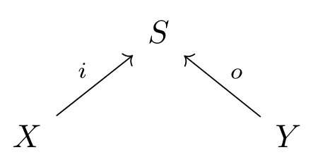
together with a vector field vv on ℝ S\mathbb{R}^S. Here the legs of the cospan mark the species that we’re allowed to inject and remove, labeled ii (oo) for input (output).

So, how can we build a category from this? Loosely citing a result of Fong, if the decorations of the cospan (in this case, the vector fields) can be given through a functor F:(FinSet,+)→(Set,×)F:(\mathbf{FinSet},+)\to(\mathbf{Set},\times ) that is lax monoidal, then we can form a category whose objects are finite sets, and whose morphisms are (iso classes of) decorated cospans.

Indeed, this can be done in a very natural way, and therefore gives rise to the category Dynam\mathbf{Dynam}, whose morphisms are open dynamical systems.

The black-boxing functor ▪:Dynam→Rel\blacksquare :\mathbf{Dynam}\to\mathbf{Rel}

Given a dynamical system, one of the first things we might like to do is to study its fixed points; in our case, study the concentration vectors that remain constant in time. When working with an open dynamical system, it’s clear that the amounts that we choose to inject and remove will alter the change in concentration of our species, and hence it makes sense to consider the following.

For an open dynamical system (X→iS←oY,v)(X\xrightarrow{i} S \xleftarrow{o} Y, v), together with a constant inflow I∈ℝ XI\in\mathbb{R}^X and constant outflow O∈ℝ YO\in\mathbb{R}^Y, a steady state (with inflows II and outflows OO) is a constant vector of concentrations c∈ℝ Sc\in\mathbb{R}^S such that

v(c)+i *(I)−o *(O)=0v(c)+i_{\ast} (I)-o_{\ast} (O)=0

Here i *(I)i_{\ast} (I) is the vector in ℝ S\mathbb{R}^S given by i *(I)(s)=∑ x∈X:i(x)=sI(x)i_{\ast} (I)(s)=\sum_{x\in X: i(x)=s} I(x); that is, the inflow concentration of all species as marked by the input leg of the cospan. As the authors concisely put it, “in a steady state, the inflows and outflows conspire to exactly compensate for the reaction velocities”.

Note that the inflow and outflow functions II and OO won’t affect any species not marked by the legs of the cospan, and so any steady state cc must be such that v(c)=0v(c)=0 when restricted to these inner species that we can’t reach.

What we want to do next is build a functor that, given an open dynamical system, records all possible combinations of input concentrations, output concentrations, inflows and outflows that hold in steady state. This process will be called black-boxing, since it discards information that can’t be seen at the inputs and outputs.

The black-boxing functor ▪:Dynam→Rel\blacksquare:\mathbf{Dynam}\to \mathbf{Rel} takes a finite set XX to the vector space ℝ X⊕ℝ X\mathbb{R}^X\oplus\mathbb{R}^X, and a morphism, that is, an open dynamical system f=(X→iS←oY,v)f=(X\xrightarrow{i} S \xleftarrow{o} Y, v), to the subset

▪(f)⊆ℝ X⊕ℝ X⊕ℝ Y⊕ℝ Y\blacksquare(f)\subseteq\mathbb{R}^X\oplus\mathbb{R}^X\oplus\mathbb{R}^Y\oplus\mathbb{R}^Y

▪(f)={(i *(c),I,o *(c),O):c  is a steady state with inflows  I  and outflows  O}\blacksquare(f)=\{(i^{\ast} (c),I,o^{\ast} (c),O): c   \text{ is a steady state with inflows }   I   \text{ and outflows }   O\}

where i *(c)i^{\ast} (c) is the vector in ℝ X\mathbb{R}^X defined by i *(c)(x)=c(i(x))i^{\ast} (c) (x)=c(i(x)); that is, the concentration of the input species.

The authors prove that black-boxing is indeed a functor, which implies that if we want to study the steady states of a complex open dynamical system, we can break it up into smaller, simpler pieces and study their steady states. In other words, studying the steady states of a big system, which is given by the composition of smaller systems (as morphisms in the category Dynam\mathbf{Dynam}) amounts to studying the steady states of each of the smaller systems, and composing them (as morphisms in Rel\mathbf{Rel}).

Spivak’s approach

The category 𝒲\mathcal{W} of wiring diagrams

Instead of dealing with dynamical systems from the start, Spivak takes a step back and develops a syntax for boxes, which are things that admit inputs and outputs.

Let’s define the category 𝒲 𝒞\mathcal{W}_\mathcal{C} of 𝒞\mathcal{C}-boxes and wiring diagrams, for a category 𝒞\mathcal{C} with finite products. Its objects are pairs

X=(X in,X out)X=(X^\text{in},X^\text{out})

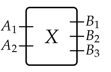
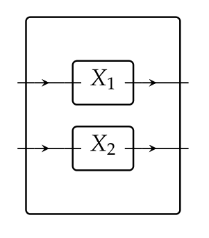
where each of these coordinates is a finite product of objects of 𝒞\mathcal{C}. For example, we interpret the pair (A 1×A 2,B 1×B 2×B 3)(A_1\times A_2, B_1\times B_2\times B_3) as a box with input ports (a 1,a 2)∈A 1×A 2(a_1 ,a_2)\in A_1\times A_2 and output ports (b 1,b 2,b 3)∈B 1×B 2×B 3(b_1 ,b_2 ,b_3 )\in B_1\times B_2\times B_3.

Its morphisms are wiring diagrams φ:X→Y\varphi:X\to Y, that is, pairs of maps (φ in,φ out)(\varphi^\text{in},\varphi^\text{out}) which we interpret as a rewiring of the box XX inside of the box YY. The function φ in\varphi^\text{in} indicates whether an input port of XX should be attached to an input of YY or to an output of XX itself; the function φ out\varphi^\text{out} indicates how the outputs of XX feed the outputs of YY. Examples of wirings are

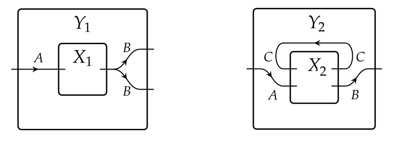
Composition is given by a nesting of wirings.

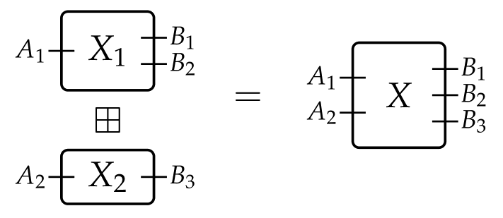
Given boxes XX and YY, we define their parallel composition by

X⊠Y=(X in×Y in,X out×Y out)X\boxtimes Y=(X^\text{in}\times Y^\text{in},X^\text{out}\times Y^\text{out})

This gives a monoidal structure to the category 𝒲 𝒞\mathcal{W}_\mathcal{C}. Parallel composition is true to its name, as illustrated by

The huge advantage of this approach is that one can now fill the boxes with suitable “inhabitants”, and model many different situations that look like wirings at their core. These inhabitants will be given through functors 𝒲 𝒞→Set\mathcal{W}_\mathcal{C}\to\mathbf{Set}, taking a box to the set of its desired interpretations, and giving a meaning to the wiring of boxes.

The functor ODS:𝒲 Euc→SetODS:\mathcal{W}_{\mathbf{Euc}}\to\mathbf{Set} of open dynamical systems

The first of our inhabitants will be, as you probably guessed by now, open dynamical systems. Here 𝒞=Euc\mathcal{C}=\mathbf{Euc} is the category of Euclidean spaces ℝ n\mathbb{R}^n and smooth maps.

From the perspective of Spivak’s paper, an (ℝ X,ℝ Y)(\mathbb{R}^X,\mathbb{R}^Y)-open dynamical system is a 3-tuple (ℝ S,f dyn,f rdt)(\mathbb{R}^S,f^\text{dyn},f^\text{rdt}) where

• ℝ S\mathbb{R}^S is the state space

• f dyn:ℝ X×ℝ S→ℝ Sf^\text{dyn}:\mathbb{R}^X\times\mathbb{R}^S\to\mathbb{R}^S is a vector field parametrized by the inputs ℝ X\mathbb{R}^X, giving the differential equation of the system

• f rdt:ℝ S→ℝ Yf^\text{rdt}:\mathbb{R}^S\to\mathbb{R}^Y is the readout function at the outputs ℝ Y\mathbb{R}^Y.

One should notice the similarity with our previously defined dynamical systems, although it’s clear that the two definitions are not equivalent.

The functor ODS:𝒲 Euc→SetODS:\mathcal{W}_{\mathbf{Euc}}\to\mathbf{Set} exhibiting dynamical systems as inhabitants of input-output boxes, takes a box X=(X in,X out)X=(X^\text{in},X^\text{out}) to the set of all (ℝ X in,ℝ X out)(\mathbb{R}^{X^\text{in}},\mathbb{R}^{X^\text{out}})-dynamical systems

ODS(X)={(ℝ S,f dyn:ℝ X in×ℝ S→ℝ S,f rdt:ℝ S→ℝ X out)}ODS(X)=\{(\mathbb{R}^S,f^\text{dyn}:\mathbb{R}^{X^\text{in}}\times\mathbb{R}^S\to\mathbb{R}^S,f^\text{rdt}:\mathbb{R}^S\to\mathbb{R}^{X^\text{out}})\}

You can surely figure out how ODSODS acts on wirings by drawing a picture and doing a bit of careful bookkeeping.

Note that there’s a natural notion of parallel composition of two dynamical systems, which amounts to carrying out the processes indicated by the two dynamical systems in parallel. Spivak shows that ODSODS is a functor, and, furthermore, that

ODS(X⊠Y)≃ODS(X)⊠ODS(Y)ODS(X\boxtimes Y)\simeq ODS(X)\boxtimes ODS(Y)

The functor Mat:𝒲 𝒞→SetMat:\mathcal{W}_{\mathcal{C}}\to\mathbf{Set} of Set\mathbf{Set}-matrices

Our second inhabitants will be given by matrices of sets. For objects X,YX,Y, an (X,Y)(X,Y)-matrix of sets is a function MM that assigns to each pair (x,y)(x,y) a set M x,yM_{x,y}. In other words, it is a matrix indexed by X×YX\times Y that, instead of coefficients, has sets in each position.

The functor Mat:𝒲 𝒞→SetMat:\mathcal{W}_{\mathcal{C}}\to\mathbf{Set} exhibiting Set\mathbf{Set}-matrices as inhabitants of input-output boxes, takes a box X=(X in,X out)X=(X^\text{in},X^\text{out}) to the set of all (X in,X out)(X^\text{in},X^\text{out})-matrices of sets

Mat(X)={{M i,j} X in×X out:M i,j  is a set}Mat(X)=\{\{M_{i,j}\}_{X^\text{in}\times X^\text{out}} : M_{i,j}   \text{ is a set}\}

Once again, it’s not too hard to figure out how MatMat should act on wirings.

Like before, there’s a notion of parallel composition of two matrices of sets, and the author shows that MatMat is a functor such that

Mat(X⊠Y)≃Mat(X)⊠Mat(Y)Mat(X\boxtimes Y)\simeq Mat(X)\boxtimes Mat(Y)

The steady-state natural transformation Stst:ODS→MatStst:ODS\to Mat

Finally, we explain how to use all this to study steady states of dynamical systems.

Given an (ℝ X,ℝ Y)(\mathbb{R}^X,\mathbb{R}^Y)-dynamical system f=(ℝ S,f dyn,f rdt)f=(\mathbb{R}^S,f^\text{dyn},f^\text{rdt}) and an element (I,O)∈ℝ X×ℝ Y(I,O)\in\mathbb{R}^X\times\mathbb{R}^Y, an (I,O)(I,O)-steady state is a state c∈ℝ Sc\in\mathbb{R}^S such that

f dyn(I,c)=0   and   f rdt(c)=Of^\text{dyn}(I,c)=0     \text{ and }     f^\text{rdt}(c)=O

Since dynamical systems are encoded by the functor ODSODS, it makes sense to study steady states through a natural transformation out of ODSODS. We define Stst:ODS→MatStst:ODS\to Mat as the transformation that assigns to each box XX, the function

Stst X:ODS(X)⟶Mat(X)Stst_X:ODS(X)\longrightarrow Mat(X)

taking a dynamical system (ℝ S,f dyn,f rdt)(\mathbb{R}^S,f^\text{dyn},f^\text{rdt}) to its matrix of steady states

M I,O={c∈ℝ S:f dyn(I,c)=0, f rdt(c)=O}M_{I,O}=\{c\in\mathbb{R}^S : f^\text{dyn}(I,c)=0,   f^\text{rdt}(c)=O\}

where (I,O)∈ℝ X in×ℝ X out(I,O)\in \mathbb{R}^{X^\text{in}}\times \mathbb{R}^{X^\text{out}}. The author proceeds to show that StstStst is a monoidal natural transformation.

Is it possible to use this machinery to draw the same conclusion as before, that is, that the steady states of a composition of systems comes from the composition of the steady states of the parts?

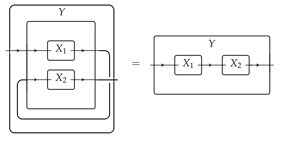
Indeed, it is! Given two boxes X 1X_1 and X 2X_2, we recover the usual notion of (serial) composition by first setting them in parallel X 1⊠X 2X_1 \boxtimes X_2,

and wiring this by φ:X 1⊠X 2→Y\varphi:X_1 \boxtimes X_2\to Y as follows:

The fact that StstStst is a monoidal natural transformation, combined with the facts that the functors ODSODS and MatMat respect parallel composition, allows us to write the following diagram, where both squares are commutative

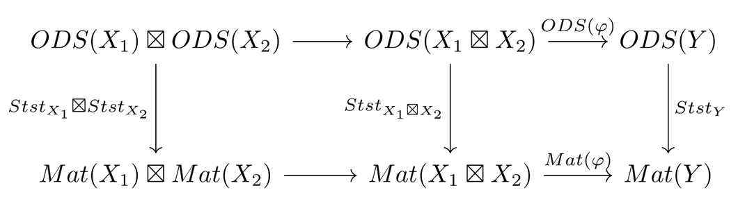
Then, chasing the diagram along the top and left sides gives the steady states of the serial composition of the dynamical systems X 1X_1 and X 2X_2, while chasing it along the right and bottom sides gives the composition of the steady states of X 1X_1 and of X 2X_2, and the two must agree.

The two approaches, side by side

So how are these two perspectives related? Looking at the definitions we can immediately see that Spivak’s approach has a broader scope than Baez and Pollard’s, so it’s apparent that his results won’t be implied by theirs.

For the converse direction, recall that in the first paper, a dynamical system is given by a decorated cospan f=(X→iS←oY,v)f=(X\xrightarrow{i} S \xleftarrow{o} Y, v), and a steady state with inflows II and outflows OO is a constant vector of concentrations c∈ℝ Sc\in\mathbb{R}^S such that

v(c)+i *(I)−o *(O)=0v(c)+i_{\ast} (I)-o_{\ast} (O)=0

Thus, studying the steady states for this cospan system corresponds to studying the box system

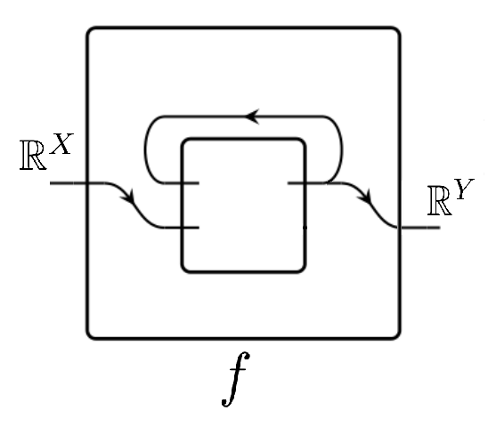
f=(ℝ S,f dyn:ℝ X×ℝ S→ℝ S,f rdt:ℝ S→ℝ Y)f=(\mathbb{R}^S, f^\text{dyn}:\mathbb{R}^X\times\mathbb{R}^S\to\mathbb{R}^S, f^\text{rdt}:\mathbb{R}^S\to\mathbb{R}^Y)

with dynamics given by f dyn(I,c)=v(c)+i *(I)−o *(f rdt(c))f^\text{dyn}(I,c)=v(c)+i_{\ast} (I)-o_{\ast} (f^\text{rdt}(c)), since its (I,O)(I,O)-steady states are vectors c∈ℝ Sc\in\mathbb{R}^S such that

f dyn(I,c)=0   and   f rdt(c)=Of^\text{dyn}(I,c)=0     \text{ and }     f^\text{rdt}(c)=O

Thus, the study of the steady states of a given cospan dynamical system can be done just as well by looking at it as a box dynamical system and running it through Spivak’s machinery. However, setting two such box systems in serial composition will not yield the box system representing the composition of the cospan systems as one would (naively?) hope, so it doesn’t seem that Spivak’s compositional results will imply those of Baez and Pollard.

This is a bit disconcerting, but instead of it being discouraging, I believe it should be seen as an invitation to delve into the semantics of open dynamical systems and find the right perspective, which manages to subsume both of the approaches presented here.

A molecule that manufactures asymmetry

A molecule that manufactures asymmetry, Published online: 10 April 2018; doi:10.1038/d41586-018-04256-4

Compound’s variations could spawn catalysts that favour certain chiral forms.

The free energy principle is the theory that the brain manipulates a probabilistic generative model of its sensory inputs, which it tries to optimize by either changing the model (learning) or changing the inputs (action) (Friston 2009; Friston 2010). The “free energy” is related to the error between predictions and actual inputs, or “surprise”, which the organism wants to minimize. It has a more precise mathematical formulation, but the conceptual issues I want to discuss here do not depend on it.

Thus, it can be seen as an extension of the Bayesian brain hypothesis that accounts for action in addition to perception. It shares the conceptual problems of the Bayesian brain hypothesis, namely that it focuses on statistical uncertainty, inferring variables of a model (called “causes”) when the challenge is to build and manipulate the structure of the model. It also shares issues with the predictive coding concept, namely that there is a conflation between a technical sense of “prediction” (expectation of the future signal) and a broader sense that is more ecologically relevant (if I do X, then Y will happen). In my view, these are the main issues with the free energy principle. Here I will focus on an additional issue that is specific of the free energy principle.

The specific interest of the free energy principle lies in its formulation of action. It resonates with a very important psychological theory called cognitive dissonance theory. That theory says that you try to avoid dissonance between facts and your system of beliefs, by either changing the beliefs in a small way or avoiding the facts. When there is a dissonant fact, you generally don’t throw your entire system of beliefs: rather, you alter the interpretation of the fact (think of political discourse or in fact, scientific discourse). Another strategy is to avoid the dissonant facts: for example, to read newspapers that tend to have the same opinions as yours. So there is some support in psychology for the idea that you act so as to minimize surprise.

Thus, the free energy principle acknowledges the circularity of action and perception. However, it is quite difficult to make it account for a large part of behavior. A large part of behavior is directed towards goals; for example, to get food and sex. The theory anticipates this criticism and proposes that goals are ingrained in priors. For example, you expect to have food. So, for your state to match your expectations, you need to seek food. This is the theory’s solution to the so-called “dark room problem” (Friston et al., 2012): if you want to minimize surprise, why not shut off stimulation altogether and go to the closest dark room? Solution: you are not expecting a dark room, so you are not going there in the first place.

Let us consider a concrete example to show that this solution does not work. There are two kinds of stimuli: food, and no food. I have two possible actions: to seek food, or to sit and do nothing. If I do nothing, then with 100% probability, I will see no food. If I seek food, then with, say, 20% probability, I will see food.

Let’s say this is the world in which I live. What does the free energy principle tell us? To minimize surprise, it seems clear that I should sit: I am certain to not see food. No surprise at all. The proposed solution is that you have a prior expectation to see food. So to minimize the surprise, you should put yourself into a situation where you might see food, ie to seek food. This seems to work. However, if there is any learning at all, then you will quickly observe that the probability of seeing food is actually 20%, and your expectations should be adjusted accordingly. Also, I will also observe that between two food expeditions, the probability to see food is 0%. Once this has been observed, surprise is minimal when I do not seek food. So, I die of hunger. It follows that the free energy principle does not survive Darwinian competition.

Thus, either there is no learning at all and the free energy principle is just a way of calling predefined actions “priors”; or there is learning, but then it doesn’t account for goal-directed behavior.

The idea to act so as to minimize surprise resonates with some aspects of psychology, like cognitive dissonance theory, but that does not constitute a complete theory of mind, except possibly of the depressed mind. See for example the experience of flow (as in surfing): you seek a situation that is controllable but sufficiently challenging that it engages your entire attention; in other words, you voluntarily expose yourself to a (moderate amount of) surprise; in any case certainly not a minimum amount of surprise.

Distortions of self-experience are critical symptoms of psychiatric disorders and have detrimental effects on social interactions. In light of the immense need for improved and targeted interventions for social impairments, it is important to better understand the neurochemical substrates of social interaction abilities. We therefore investigated the pharmacological and neural correlates of self- and other-initiated social interaction. In a double-blind, randomized, counterbalanced, crossover study 24 healthy human participants (18 males and 6 females) received either (1) placebo + placebo, (2) placebo + lysergic acid diethylamide (LSD; 100 μg, p.o.), or (3) ketanserin (40 mg, p.o.) + LSD (100 μg, p.o.) on three different occasions. Participants took part in an interactive task using eye-tracking and functional magnetic resonance imaging completing trials of self- and other-initiated joint and non-joint attention. Results demonstrate first, that LSD reduced activity in brain areas important for self-processing, but also social cognition; second, that change in brain activity was linked to subjective experience; and third, that LSD decreased the efficiency of establishing joint attention. Furthermore, LSD-induced effects were blocked by the serotonin 2A receptor (5-HT_2AR) antagonist ketanserin, indicating that effects of LSD are attributable to 5-HT_2AR stimulation. The current results demonstrate that activity in areas of the "social brain" can be modulated via the 5-HT_2AR thereby pointing toward this system as a potential target for the treatment of social impairments associated with psychiatric disorders.

SIGNIFICANCE STATEMENT Distortions of self-representation and, potentially related to this, dysfunctional social cognition are central hallmarks of various psychiatric disorders and critically impact disease development, progression, treatment, as well as real-world functioning. However, these deficits are insufficiently targeted by current treatment approaches. The administration of lysergic acid diethylamide (LSD) in combination with functional magnetic resonance imaging and real-time eye-tracking offers the unique opportunity to study alterations in self-experience, their relation to social cognition, and the underlying neuropharmacology. Results demonstrate that LSD alters self-experience as well as basic social cognition processing in areas of the "social brain". Furthermore, these alterations are attributable to 5-HT_2A receptor stimulation, thereby pinpointing toward this receptor system in the development of pharmacotherapies for sociocognitive deficits in psychiatric disorders.

Our sensors give us an incomplete, noisy, and indirect information about the world. For example, estimating the location of a sound source is difficult because in natural contexts, the sound of interest is corrupted by other sound sources, reflections, etc. Thus it is not possible to know the position of the source with certainty. The ‘Bayesian coding hypothesis’ (Knill & Pouget, 2014) postulates that the brain represents not the most likely position, but the entire probability distribution of the position. It then uses those distributions to do Bayesian inference, for example, when combining different sources of information (say, auditory and visual). This would allow the brain to optimally infer the most likely position. There is indeed some evidence for optimal inference in psychophysical experiments – although there is also some contradicting evidence (Rahnev & Denison, 2018).

The idea has some appeal. The problem is that, by framing perception as a statistical inference problem, it focuses on the most trivial type of uncertainty, statistical uncertainty. It is illustrated by the following quote: “The fundamental concept behind the Bayesian approach to perceptual computations is that the information provided by a set of sensory data about the world is represented by a conditional probability density function over the set of unknown variables”. Implicit in this representation is a particular model, for which variables are defined. Typically, one model describes a particular experimental situation. For example, the model would describe the distribution of auditory cues associated with the position of the sound source. Another situation would be described by a different model, for example one with two sound sources would require a model with two variables. Or if the listening environment is a room and the size of that room might vary, then we would need a model with the dimensions of the room as variables. In any of these cases where we have identified and fixed parametric sources of variation, then the Bayesian approach works fine, because we are indeed facing a problem of statistical inference. But that framework doesn’t fit any real life situation. In real life, perceptual scenes have variable structure, which corresponds to the model in statistical inference (there is one source, or two sources, we are in a room, the second source comes from the window, etc). The perceptual problem is therefore not just to infer the parameters of the model (dimensions of the room etc), but also the model itself, its structure. Thus, it is not possible in general to represent an auditory scene by a probability distribution on a set of parameters, because the very notion of a parameter already assumes that the structure of the scene is known and fixed.

Inferring parameters for a known statistical model is relatively easy. What is really difficult, and is still challenging for machine learning algorithms today, is to identify the structure of a perceptual scene, what constitutes an object (object formation), how objects are related to each other (scene analysis). These fundamental perceptual processes do not exist in the Bayesian brain. This touches on two very different types of uncertainty: statistical uncertainty, variations that can be interpreted and expected in the framework of a model; and epistemic uncertainty,  the model is unknown (the difference has been famously explained by Donald Rumsfeld).

Thus, the “Bayesian brain” idea addresses an interesting problem (statistical inference), but it trivializes the problem of perception, by missing the fact that the real challenge is epistemic uncertainty (building a perceptual model), not statistical uncertainty (tuning the parameters): the world is not noisy, it is complex.

We argue that dualities offer new possibilities for relating fundamentality, levels, and emergence. Namely, dualities often relate two theories whose hierarchies of levels are inverted relative to each other, and so allow for new fundamentality relations, as well as for epistemic emergence. We find that the direction of emergence typically found in these cases is opposite to the direction of emergence followed in the standard accounts. Namely, the standard emergence direction is that of decreasing fundamentality: there is emergence of less fundamental, high-level entities, out of more fundamental, low-level entities. But in cases of duality, a more fundamental entity can emerge out of a less fundamental one. This possibility can be traced back to the existence of different classical limits in quantum field theories and string theories.

Arizona rolled out the regulation-free welcome mat after California basically kicked Uber out because Uber didn't think minimal "regulations" or "safety measures" applied to them.

After a fairly seamless, high-profile launch in Pittsburgh, the rollout in San Francisco was bumpy right from the beginning. First, the DMV issued a warning to Uber that it had not obtained the proper testing permits for its pilot program. Then, a few hours after the trial began, The Verge reported that one of Uber’s cars ran a red light, nearly hitting a (human-driven) Lyft car.


Uber reviewed the case and determined it was actually the fault of the human driver sitting in the car—remember, Uber still has human drivers who can “take over” from the self-driving system as needed.

Then there was the bike lane problem. Uber’s vehicles had a nasty habit of driving into San Francisco’s bike lanes without warning. This was not the fault of humans but a software error, claimed Uber, noting that the problem had not come up in Pittsburgh, which also has a robust cycling network. Uber pledged to fix it.

Wasn't that long ago:

Arizona has since built upon the governor’s action to become a favored partner for the tech industry, turning itself into a live laboratory for self-driving vehicles. Over the past two years, Arizona deliberately cultivated a rules-free environment for driverless cars, unlike dozens of other states that have enacted autonomous vehicle regulations over safety, taxes and insurance.

...

Mr. Ducey, a native of Ohio who came to Arizona for college and then stayed, was elected governor in 2014 on a pro-business and innovation platform. He quickly lifted restrictions on medical testing for companies like Theranos, a Silicon Valley company that later faced scrutiny for its business practices. He also touted Apple’s decision to build a $2 billion data center in the state.

“We can beat California in every metric; lower taxes, less regulations, cost of living, quality of life,” he said several months after he became governor.

Oh well.

PHOENIX, Ariz., March 26 (Reuters) - The governor of Arizona on Monday suspended Uber’s ability to test self-driving cars on public roads in the state following a fatal crash last week that killed a 49-year-old woman pedestrian.

In a letter sent to Uber Chief Executive Dara Khosrowshahi and shared with the media, Governor Doug Ducey said he found a video released by police of the crash “disturbing and alarming, and it raises many questions about the ability of Uber to continue testing in Arizona.”

Good calls, bro. All of them.

...I wrote this last night, but the local fishwrap is on it, also, too.

Author(s): Kiyoshi Kanazawa, Takumi Sueshige, Hideki Takayasu, and Misako Takayasu

Using data on the activity of individual financial traders, researchers have devised a microscopic financial model that can explain macroscopic market trends.

[Phys. Rev. Lett. 120, 138301] Published Tue Mar 27, 2018

The post Iranian “CyberAttack” Threatens Elsevier Not USA appeared first on Marginal REVOLUTION.

A couple of years ago I was reading Wikipedia's article about the the 1943 Bengal famine, and I was startled by the following claim:

"If food is so scarce, why hasn’t Gandhi died yet?"

Winston Churchill's response to an urgent request to release food stocks for India.

It was cited, but also marked with the “not in citation” tag, which is supposed to mean that someone checked the reference and found that it did not actually support the claim.

It sounded like it might be the sort of scurrilous lie that is widely repeated but not actually supportable, so I went to follow it up. It turned out that although the quotation was not quite exact, it was not misleadingly altered, and not a scurrilous lie at all. The attributed source (Tharoor, Shashi "The Ugly Briton". Time, (29 November 2010).) claimed:

Churchill's only response to a telegram from the government in Delhi about people perishing in the famine was to ask why Gandhi hadn't died yet.

I removed the “not in citation” tag, which I felt was very misleading.

Still, I felt that anything this shocking should be as well-supported as possible. It cited Tharoor, but Tharoor could have been mistaken. So I put in some effort and dug up the original source. It is from the journal entry of Archibald Wavell, then Viceroy of India, of 5 July 1944:

Winston sent me a peevish telegram to ask why Gandhi hadn't died yet! He has never answered my telegram about food.

This appears in the published version of Lord Wavell's journals. (Wavell, Archibald Percival. Wavell: The Viceroy's journal, p. 78. Moon, Penderel, ed. Oxford University Press, 1973.) This is the most reliable testimony one could hope for. The 1973 edition is available from the Internet Archive.

A few months later, the entire article was massively overhauled by a group of anglophiles and Churchill-rehabilitators. Having failed to remove the quotation for being uncited, and then having failed to mendaciously discredit the cited source, they removed the quotation in a typical episode of Wikipedia chicanery. In a 5,000-word article, one sentence quoting the views of the then-current British Prime Minister was deemed “undue weight”, and a failure to “fairly represent all significant viewpoints that have been published by reliable sources”.

Further reading: In Winston Churchill, Hollywood rewards a mass murderer. (Tharoor again, in last week's Washington Post.)

Chris just sent me the following:

Hi Igor-
I hope you are well. I wanted to alert you that our paper on delay-coordinate maps and Takens' embeddings has finally appeared.
Eftekhari, Armin, Han Lun Yap, Michael B. Wakin, and Christopher J. Rozell. "Stabilizing embedology: Geometry-preserving delay-coordinate maps." Physical Review E 97, no. 2 (2018): 022222.
http://dx.doi.org/10.1103/PhysRevE.97.022222
preprint:
http://arxiv.org/pdf/1609.06347
You had mentioned a much earlier preliminary result on your blog but this is the full and final result. It uses the tools familiar to this community (random measurements, stable embeddings) to address a fundamental observability result about nonlinear (perhaps even chaotic) dynamical systems from the physics community. The key question is "how much information is there in a time series measurement about the dynamical system that created it?". I think this result is a unique convergence of different fields, and our previous results analyzing recurrent neural networks were a distinct outgrowth of working on this problem.
regards,
chris

Delay-coordinate mapping is an effective and widely used technique for reconstructing and analyzing the dynamics of a nonlinear system based on time-series outputs. The efficacy of delay-coordinate mapping has long been supported by Takens' embedding theorem, which guarantees that delay-coordinate maps use the time-series output to provide a reconstruction of the hidden state space that is a one-to-one embedding of the system's attractor. While this topological guarantee ensures that distinct points in the reconstruction correspond to distinct points in the original state space, it does not characterize the quality of this embedding or illuminate how the specific parameters affect the reconstruction. In this paper, we extend Takens' result by establishing conditions under which delay-coordinate mapping is guaranteed to provide a stable embedding of a system's attractor. Beyond only preserving the attractor topology, a stable embedding preserves the attractor geometry by ensuring that distances between points in the state space are approximately preserved. In particular, we find that delay-coordinate mapping stably embeds an attractor of a dynamical system if the stable rank of the system is large enough to be proportional to the dimension of the attractor. The stable rank reflects the relation between the sampling interval and the number of delays in delay-coordinate mapping. Our theoretical findings give guidance to choosing system parameters, echoing the trade-off between irrelevancy and redundancy that has been heuristically investigated in the literature. Our initial result is stated for attractors that are smooth submanifolds of Euclidean space, with extensions provided for the case of strange attractors.

The 2018 Abel Prize has been awarded to Robert Langlands, an excellent choice. The so-called “Langlands program” has been a huge influence on modern mathematics, providing deep insight into the structure of number theory while linking together disparate fields of mathematics, as well as quantum field theories and physics.

The Abel Prize site provides a wealth of information about Langlands and his work. Davide Castelvecchi at Nature appropriately describes the Langlands program as a “grand unified theory of mathematics” (Edward Frenkel’s Love and Math popularized this description).

Many blog posts here have discussed the Langlands program and ideas that have developed out of it. For a good example of how wide the impact of these ideas has been, this week the Perimeter Institute will be hosting a conference discussing the latest work on the geometric version of the Langlands program, as well as connections to gauge theory and conformal field theory.

For the original work of Langlands himself, besides the material at the Abel site, the AMS Bulletin has recently published a long article by Julia Mueller. For the original sources and a wealth of other material written by Langlands himself, see the IAS site that collects his writings.

There were the evil bastards, and then there were the Model UN debate team crowd, young boy blunders putting on their first big boy suits writing for big boy magazines and being on big boy teevee shows, being patted on the head for punching hippies. War was very serious, they intoned, and only the Very Serious People could be trusted with it. It must have been so exciting!

No one knows for certain how many Iraqis have died as a result of the invasion 15 years ago. Some credible estimates put the number at more than one million. You can read that sentence again. The invasion of Iraq is often spoken of in the United States as a “blunder,” or even a “colossal mistake.” It was a crime. Those who perpetrated it are still at large. Some of them have even been rehabilitated thanks to the horrors of Trumpism and a mostly amnesiac citizenry. (A year ago, I watched Mr. Bush on “The Ellen DeGeneres Show,” dancing and talking about his paintings.) The pundits and “experts” who sold us the war still go on doing what they do. I never thought that Iraq could ever be worse than it was during Saddam’s reign, but that is what America’s war achieved and bequeathed to Iraqis.

In Sheffield we have started a reading seminar on the recent paper of Tom Leinster and Mike Shulman Magnitude homology of enriched categories and metric spaces. The plan was to write the talks up as blog posts. Various things, including the massive strike that has been going on in universities in the UK, have meant that I’m somewhat behind with putting the first talk up. The strike also means that we haven’t had many seminars yet!

I gave the first talk which is the one here. It is an introductory talk which just describes the idea of categorification and the paper I wrote with Richard Hepworth on categorifying the magnitude of finite graphs, this is the idea which was generalized by Tom and Mike.

Categorification

Categorification means many things. In this context it is supposed to be the idea of lifting an invariant from taking values in a set to values in a category. Let’s look at two examples.

[This is possibly a caricature of what actually happened. It would be nice to have some references!] In the eighteenth century, mathematicians such as Riemann knew about the Euler characteristic of surfaces (and possibly manifolds). This is a fundamental invariant which seems to crop up in all sorts of places. Towards the end of the century Poincar'e introduced homology groups H ⋆(M)\text{H}_\star(M) of a manifold MM and was aware

χ(M)=rank(H ⋆(M))=∑ i(−1) irank(H i(M)). \chi(M)=rank(\text{H}_\star(M))= \sum_i (-1)^i rank (\text{H}_i(M)).

I get the impression the functorial nature of homology was not appreciated until later, but this adds another layer of structure.

Around 1985 Jones introduced his eponymous polynomial J(L)∈ℤ[q ±1]\text{J}(L)\in \mathbb{Z}[q^{\pm 1}] for a knot or link LL in 33-space. This gives a polynomial invariant of links. In around 1999, Khovanov introduced Khovanov homology Kh ⋆,⋆(L)Kh_{\star, \star}(L) for a link LL, this is bigraded group. The Jones polynomial is obtained from it by taking the dimension (or Euler characteristic!) in an appropriate graded sense:

J(L)=∑ i,j(−1) iq jrank(Kh i,j(L)). \text{J}(L)= \sum_{i,j} (-1)^i q^j rank( Kh_{i,j}(L)).

In both these cases we lift an invariant which takes values in a set (either ℤ\mathbb{Z} or ℤ[q ±1] \mathbb{Z}[q^{\pm 1}]) to an invariant which takes values in a category (either graded groups or bigraded groups). This lifted invariant has a richer structure and functorial properties, but is probably harder to calculate! This is what we mean by categorifying an invariant.

Magnitude of enriched categories

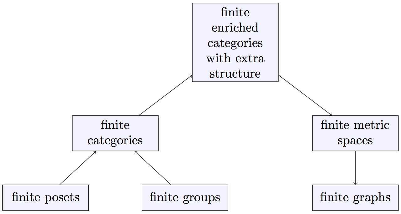
There was a classical notion of Euler characteristic for finite groups and also one for finite posets. We know that finite groups and finite posets are both examples of finite categories (at one extreme with only one object and at the other extreme with at most one morphism between each pair of objects). Tom found a common generalization of these Euler characteristics which is the idea of an Euler characteristic for finite categories (we will see the definition next week). He further generalized that to the notion of an Euler characteristic for enriched categories (with a additional bit of structure, wait for next week). Finite metric spaces are examples of enriched categories and so have a notion of Euler characteristic. We decided the name was too confusing so after consulting a thesaurus we decided on “magnitude” (having toyed with the name “cardinality”). Tom later noticed something nice about the magnitude of the metric spaces that you get from finite graphs (partly because these have integer-valued metrics).

The journey from the Euler characteristics of finite posets and finite groups to the magnitude of finite graphs via a sequence of generalizations and specializations can be viewed as a trip up and then down the following picture.

Magnitude of metric spaces (more next week)

For X={x 1,…x n}X=\{x_1,\dots x_n\} a finite metric space with the metric we can define a matrix ZZ by Z i,j=e −d(x i,x j)Z_{i,j}=e^{-\text{d}(x_i,x_j)}. The magnitude |X||X| is defined to be the sum of the entries of the inverse matrix (if it exists): |X|:=∑ i,j(Z −1) i,j|X|:=\sum_{i,j}(Z^{-1})_{i,j}. It is actually more interesting if we look at what happens as we scale XX (or perhaps if we introduce an indeterminate into the metric). For t>0t> 0, we define t⋅Xt\cdot X to have the same underlying set, but with the metric scaled by a factor of tt. This gives us the magnitude function |t⋅X|\left|t\cdot X\right| which is a function of tt.

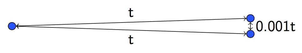
We can have a look at a simple example where we take XX to be a three-point metric space in which two points are much, much closer to each other than they are to the third point. Here is a picture of t⋅Xt\cdot X.

Here is the graph of the magnitude function of the metric space XX.

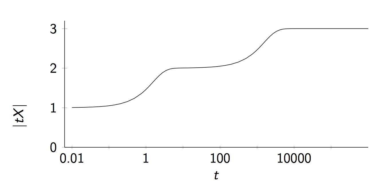
This shows in some sense how the magnitude can be viewed as an “effective number of points”. At small scales there is effectively one point, at middling scales there is effectively two points and at very large scales there are effectively three points.

Although the definition looks rather ad hoc, it turns out that it has various connections to thinks like measurements of biodiversity, Hausdorff dimension, volumes, potential theory and several other fun things.

Magnitude of graphs

Suppose that GG is a finite graph, then it gives rise to a finite metric space (which we will also write as GG) which has the vertices of GG as its points and the shortest path distance as its metric, where all edges have length one.

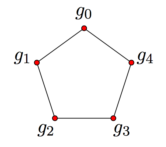
For example we have the five-cycle graph below with d(g 0,g 3)=2\text{d}(g_0, g_3)=2.

Tom noticed that we can use the magnitude function of the associated metric space to get an integral power series from the graph. Firstly, we can write q=e −tq=e^{-t} then the entries of the matrix ZZ are just integer powers of qq as all of the distances in GG are integral. This means that the entries of Z −1Z^{-1} are just rational functions of qq (with integer coefficients) and hence so is their sum, the magnitude function. Moreover the denominator of this rational function is the determinant of ZZ which, as the diagonal entries of ZZ are all e 0e^{0}, i.e., 11, is of the form 1+powers of q1+\text{powers of }q. So we can take a power series expansion of |t⋅G||t\cdot G| to get an integer power series in q=e −tq=e^{-t}. We denote this power series by #G\# G.

For example, for the five-cycle graph C 5C_5 pictured above we have

#C 5=5−10q+10q 2−20q 4+40q 5−40q 6+⋯. \# C_5 = 5-10q+10q^2-20q^4+40q^5-40q^6+\cdots.

In general we can identify the first two coefficients as the number of vertices and −2-2 times the number of edges, respectively.

Categorifying the magnitude of graphs

As Richard Hepworth noticed, we can categorify this! In other words, we can find a homology theory which has the magnitude power series #G∈Z[q]\# G\in \Z[q] as its graded Euler characteristic.

For a finite graph GG define the magnitude chain groups as follows.

MC k,l(G)=⟨(x 0,…,x k)|x i−1≠x i,∑dd(x i−1,x i)=l⟩. MC_{k,l}(G)=\left\langle (x_0,\dots, x_k) \big | x_{i-1}\ne x_{i},\quad \sum \dd(x_{i-1}, x_i)=l\right\rangle.

For example a chain group generator for the five-cycle graph from above is (g 0,g 1,g 2,g 4,g 2)∈MC 4,6(C 5)(g_0, g_1, g_2, g_4, g_2)\in MC_{4,6}(C_5).

We define maps ∂ i:MC k,l(G)→MC k−1,l(G)\partial_i\colon MC_{k,l}(G)\to MC_{k-1,l}(G) for i=1,…,k−1i=1,\dots, k-1:

∂ i(x 0,…,x k)={(x 0,…,x i^,…,x k) ifx i−1<x i<x i+1, 0 otherwise. \partial_{i}(x_0,\ldots,x_k) = \begin{cases} (x_0,\ldots,\widehat{x_i},\ldots,x_k) & \text{if}\,\, x_{i-1}&lt;x_{i}&lt;x_{i+1}, \\ 0 & \text{otherwise}. \end{cases}

where x i−1<x i<x i+1x_{i-1}&lt;x_{i}&lt;x_{i+1} means that x ix_i lies on a shortest path between x i−1x_{i-1} and x i+1x_{i+1}, i.e., d(x i−1,x i)+d(x i,x i+1)=d(x i−1,x i+1)\text{d}(x_{i-1},x_i)+\text{d}(x_i,x_{i+1})=\text{d}(x_{i-1},x_{i+1}).

So for our example chain generator in C 5C_5 you can check that we have

∂ i(g 0,g 1,g 2,g 4,g 2)={(g 0,g 2,g 4,g 2) ifi=1, 0 otherwise. \partial_{i}(g_0, g_1, g_2, g_4, g_2) = \begin{cases} (g_0, g_2, g_4, g_2) & \text{if}\,\, i=1, \\ 0 & {otherwise}. \end{cases}

In the usual way, the differential ∂:MC k,l(G)→MC k−1,l(G)\partial\colon MC_{k,l}(G)\to MC_{k-1,l}(G) is defined as the alternating sum

∂=∂ 1−∂ 2+⋯+(−1) k−1∂ k−1. \partial=\partial_1-\partial_2+\cdots+(-1)^{k-1}\partial_{k-1}.

One can show that this is a differential, so that ∂∘∂=0\partial\circ\partial =0. Then taking homology gives what is defined to be magnitude homology groups of the graph:

MH k,l(G)=H k(MC *,l(G),∂). \MH_{k,l}(G)= \text{H}_k(\MC_{\ast,l}(G), \partial).

By direct computation you can calculate the ranks of the magnitude homology groups of the five-cycle graph. The following table shows the ranks rank(MH k,l(C 5))rank(MH_{k,l}(C_5)) for small kk and ll.

k 0 1 2 3 4 5 6 χ(MH *,l(C 5)) 0 5 5 1 10 −10 2 10 10 l 3 10 10 0 4 30 10 −20 5 50 10 40 6 20 70 10 −40 \begin{array}{rrrrrrrrrrc} &&&&&k\\ &&0&1&2&3&4&5&6&&\chi(MH_{\ast,l}(C_5))\\ &0 & 5&&&&&&&\qquad&5\\ & 1 & & 10 &&&&&&&-10 \\ &2 & && 10 &&&&&&10\\ l& 3 &&& 10 & 10 &&&&&0 \\ & 4 &&&& 30 & 10 &&&&-20\\ & 5 &&&&& 50 & 10 &&&40 \\ & 6 &&&&& 20 & 70 & 10 &&-40 \end{array}

The final column shows the Euler characteristics, which are just the alternating sums of entries in the rows. You can check that these are precisely the coefficients in the power series #C 5\# C_5 given above: this illustrates the fact that graph magnitude homology does indeed categorify graph magnitude in the sense of the following theorem.

Theorem #G=∑ k,l≥0(−1) kq lrank(MH k,l(G))∈ℤ[[q]]. \#G = \sum_{k,l\geq 0} (-1)^k q^l \,rank \bigl(MH_{k,l}(G)\bigr)\in \mathbb{Z}[[q]].

Thus we have MH *,*MH_{\ast,\ast} which a bigraded group valued invariant of graphs which is functorial with respect to certain maps of graphs and has properties like Kunneth Theorem and long exact sequences: richer but harder to calculate than the graph magnitude.

In the following weeks we will hopefully see how Mike and Tom have generalized this construction up to the top of the picture above, namely to certain enriched categories with extra structure.

Virtually all network analyses involve structural measures between pairs of vertices, or of the vertices themselves, and the large amount of symmetry present in real-world complex networks is inherited by such measures. This has practical consequences which have not yet been explored in full generality, nor systematically exploited by network practitioners. Here we study the effect of network symmetry on arbitrary network measures, and show how this can be exploited in practice in a number of ways, from redundancy compression, to computational reduction. We also uncover the spectral signatures of symmetry for an arbitrary network measure such as the graph Laplacian. Computing network symmetries is very efficient in practice, and we test real-world examples up to several million nodes. Since network models are ubiquitous in the Applied Sciences, and typically contain a large degree of structural redundancy, our results are not only significant, but widely applicable.

This justification for lack of universal coverage of [insert appropriate government function here] is just a mirror image of the "what if your tax moneys go to blah people????" that conservatives use to fight the same things. People making the argument are stupid or lying (always the question). Benefits can be universal and taxes can be progressive. The top 1% doesn't care about receiving these benefits, anyway, they just don't want to pay the taxes.

We develop a theoretical description of non-Hermitian time evolution that accounts for the break- down of the adiabatic theorem. We obtain closed-form expressions for the time-dependent state amplitudes, involving the complex eigen-energies as well as inter-band Berry connections calculated using basis sets from appropriately-chosen Schur decompositions. Using a two-level system as an example, we show that our theory accurately captures the phenomenon of "sudden transitions", where the system state abruptly jumps from one eigenstate to another.

We investigate the sensorimotor loop of simple robots simulated within the LPZRobots environment from the point of view of dynamical systems theory. For a robot with a cylindrical shaped body and an actuator controlled by a single proprioceptual neuron we find various types of periodic motions in terms of stable limit cycles. These are self-organized in the sense, that the dynamics of the actuator kicks in only, for a certain range of parameters, when the barrel is already rolling, stopping otherwise. The stability of the resulting rolling motions terminates generally, as a function of the control parameters, at points where fold bifurcations of limit cycles occur. We find that several branches of motion types exist for the same parameters, in terms of the relative frequencies of the barrel and of the actuator, having each their respective basins of attractions in terms of initial conditions. For low drivings stable limit cycles describing periodic and drifting back-and-forth motions are found additionally. These modes allow to generate symmetry breaking explorative behavior purely by the timing of an otherwise neutral signal with respect to the cyclic back-and-forth motion of the robot.

Matthew Fisher recently postulated a mechanism by which quantum phenomena could influence cognition: Phosphorus nuclear spins may resist decoherence for long times, especially when in Posner molecules. The spins would serve as biological qubits. We imagine that Fisher postulates correctly. How adroitly could biological systems process quantum information (QI)? We establish a framework for answering. Additionally, we construct applications of biological qubits to quantum error correction, quantum communication, and quantum computation. First, we posit how the QI encoded by the spins transforms as Posner molecules form. The transformation points to a natural computational basis for qubits in Posner molecules. From the basis, we construct a quantum code that detects arbitrary single-qubit errors. Each molecule encodes one qutrit. Shifting from information storage to computation, we define the model of Posner quantum computation. To illustrate the model's quantum-communication ability, we show how it can teleport information incoherently: A state's weights are teleported. Dephasing results from the entangling operation's simulation of a coarse-grained Bell measurement. Whether Posner quantum computation is universal remains an open question. However, the model's operations can efficiently prepare a Posner state usable as a resource in universal measurement-based quantum computation. The state results from deforming the Affleck-Kennedy-Lieb-Tasaki (AKLT) state and is a projected entangled-pair state (PEPS). Finally, we show that entanglement can affect molecular-binding rates, boosting a binding probability from 33.6% to 100% in an example. This work opens the door for the QI-theoretic analysis of biological qubits and Posner molecules.

guest post by Tai-Danae Bradley and Brad Theilman

Recently in the Applied Category Theory Seminar our discussions have returned to modeling natural language, this time via Interacting Conceptual Spaces I by Joe Bolt, Bob Coecke, Fabrizio Genovese, Martha Lewis, Dan Marsden, and Robin Piedeleu. In this paper, convex algebras lie at the heart of a compositional model of cognition based on Peter Gärdenfors’ theory of conceptual spaces. We summarize the ideas in today’s post.

Sincere thanks go to Brendan Fong, Nina Otter, Fabrizio Genovese, Joseph Hirsh, and other participants of the seminar for helpful discussions and feedback.

Introduction

A few weeks ago here at the Café, Cory and Jade summarized the main ideas behind the DisCoCat model, i.e. the categorical compositional distributional model of meaning developed in a 2010 paper by Coecke, Sadrzadeh, and Clark. Within the comments section of that blog entry, Coecke noted that the DisCoCat model is essentially a grammatical quantum field theory — a functor (morally) from a pregroup to finite dimensional real vector spaces. In this model, the meaning of a sentence is determined by the meanings of its constituent parts, which are themselves represented as vectors with meanings determined statistically. But as he also noted,

Vector spaces are extremely bad at representing meanings in a fundamental way, for example, lexical entailment, like tiger < big cat < mammal < animal can’t be represented in a vector space. At Oxford we are now mainly playing around with alternative models of meaning drawn from cognitive science, psychology and neuroscience. Our Interacting Conceptual Spaces I is an example of this….

This (ICS I) is the paper that we discuss in today’s blog post. It presents a new model in which words are no longer represented as vectors. Instead, they are regions within a conceptual space, a term coined by cognitive scientist Peter Gärdenfors in Conceptual Spaces: The Geometry of Thought. A conceptual space is a combination of geometric domains where convexity plays a key role. Intuitively, if we have a space representing the concept of fruit, and if two points in this space represent banana, then one expects that every point “in between” should also represent banana. The goal of ICS I is to put Gärdenfors’ idea on a more formal categorical footing, all the while adhering to the main principles of the DisCoCat model. That is, we still consider a functor out of a grammar category, namely the pregroup Preg(n,s)\mathsf{Preg}(n,s), freely generated by noun type nn and sentence type ss. (But in light of Preller’s argument as mentioned previously, we use the word functor with caution.) The semantics category, however, is no longer vector spaces but rather ConvexRel,\mathsf{ConvexRel}, the category of convex algebras and convex relations. We make these ideas and definitions precise below.

Preliminaries

A convex algebra is, loosely speaking, a set equipped with a way of taking formal finite convex combinations of its elements. More formally, let AA be a set and let D(A)D(A) denote the set of formal finite sums ∑ ip ia i\sum_i p_i a_i of elements of A,A, where p i∈ℝ ≥0p_i\in\mathbb{R}_{\geq 0} and ∑ ip i=1.\sum_i p_i=1. (We emphasize that this sum is formal. In particular, AA need not be equipped with a notion of addition or scaling.) A convex algebra is a set AA together with a function α:D(A)→A\alpha\colon D(A)\to A, called a “mixing operation,” that is well-behaved in the following sense:

• the convex combination of a single element is itself, and
• the two ways of evaluating a convex combination of a convex combination are equal.

For example, every convex subspace of ℝ n\mathbb{R}^n is naturally a convex algebra. (And we can’t resist mentioning that convex subspaces of ℝ n\mathbb{R}^n are also examples of algebras over the operad of topological simplices. But as we learned through a footnote in Tobias Fritz’s Convex Spaces I, it’s best to stick with monads rather than operads. Indeed, a convex algebra is an Eilenberg-Moore algebra of the finite distribution monad.) Join semilattices also provide an example of convex algebras. A finite convex combination of elements a ia_i in the lattice is defined to be the join of those elements having non-zero coefficients: ∑ ip ia i:=∨ i{a i:p i≠0}\sum_i p_i a_i:=\vee_i \{a_i:p_i\neq 0\}. (In particular, the coefficients play no role on the right-hand side.)

Given two convex algebras (A,α)(A,\alpha) and (B,β)(B,\beta), a convex relation is a binary relation R⊆A×BR\subseteq A\times B that respects convexity. That is, if R(a i,b i)R(a_i,b_i) for all i=1,…,ni=1,\ldots,n then R(α(∑ i=1 np ia i),β(∑ i=1 np ib i))R\left(\alpha(\sum_{i=1}^n p_i a_i),\beta(\sum_{i=1}^n p_i b_i)\right). We then define ConvexRel\mathsf{ConvexRel} to be the category with convex algebras as objects and convex relations as morphisms. Composition and identities are as for usual binary relations.

Now since in this model, the category of vector spaces is being replaced by ConvexRel\mathsf{ConvexRel}, one hopes that (in keeping with the spirit of the DisCoCat model), the latter admits a symmetric monoidal compact closed structure. Indeed it does.

• ConvexRel\mathsf{ConvexRel} has a symmetric monoidal structure given by the Cartesian product: We use (A,α)⊗(B,β)(A,\alpha)\otimes(B,\beta) to denote the set A×BA\times B equipped with mixing operation given by D(A×B) ⟶A×B ∑p i(a i,b i) ↦(α(∑p ia i),β(∑p ib i)). \begin{aligned} D(A\times B)&\longrightarrow A\times B\\ \sum p_i(a_i,b_i)&\mapsto \left(\alpha(\sum p_i a_i),\beta(\sum p_i b_i)\right). \end{aligned} The monoidal unit is the one-point set ⋆\star which has a unique convex algebra structure. We’ll denote this convex algebra by I.I.
• Each object in ConvexRel\mathsf{ConvexRel} is self-dual, and cups and caps are given as follows: η A:I→(A,α)⊗(A,α) is the relation{(⋆,(a,a)):a∈A)} ϵ A:(A,α)⊗(A,α)→I is the relation{((a,a),⋆):a∈A}\begin{aligned} \eta_A\colon I \to(A,\alpha)\otimes(A,\alpha) \quad &\text{ is the relation} \quad \{(\star,(a,a)):a\in A)\}\\ \epsilon_A\colon (A,\alpha)\otimes(A,\alpha)\to I \quad &\text{ is the relation} \quad \{((a,a),\star):a\in A\} \end{aligned}

The compact closed structure guarantees that ConvexRel\mathsf{ConvexRel} fits nicely into the DisCoCat framework: words in a sentence are assigned types according to a chosen pregroup grammar, and a sentence is deemed grammatical if it reduces to type ss. Moreover, these type reductions in Preg(n,s)\mathsf{Preg}(n,s) give rise to corresponding morphisms in ConvexRel\mathsf{ConvexRel} where the meaning of the sentence can be determined. We’ll illustrate this below by computing the meaning of the sentence

bananastastesweet. b a n a n a s\; t a s t e\; s w e e t.

To start, note that this sentence is comprised of three grammar types:

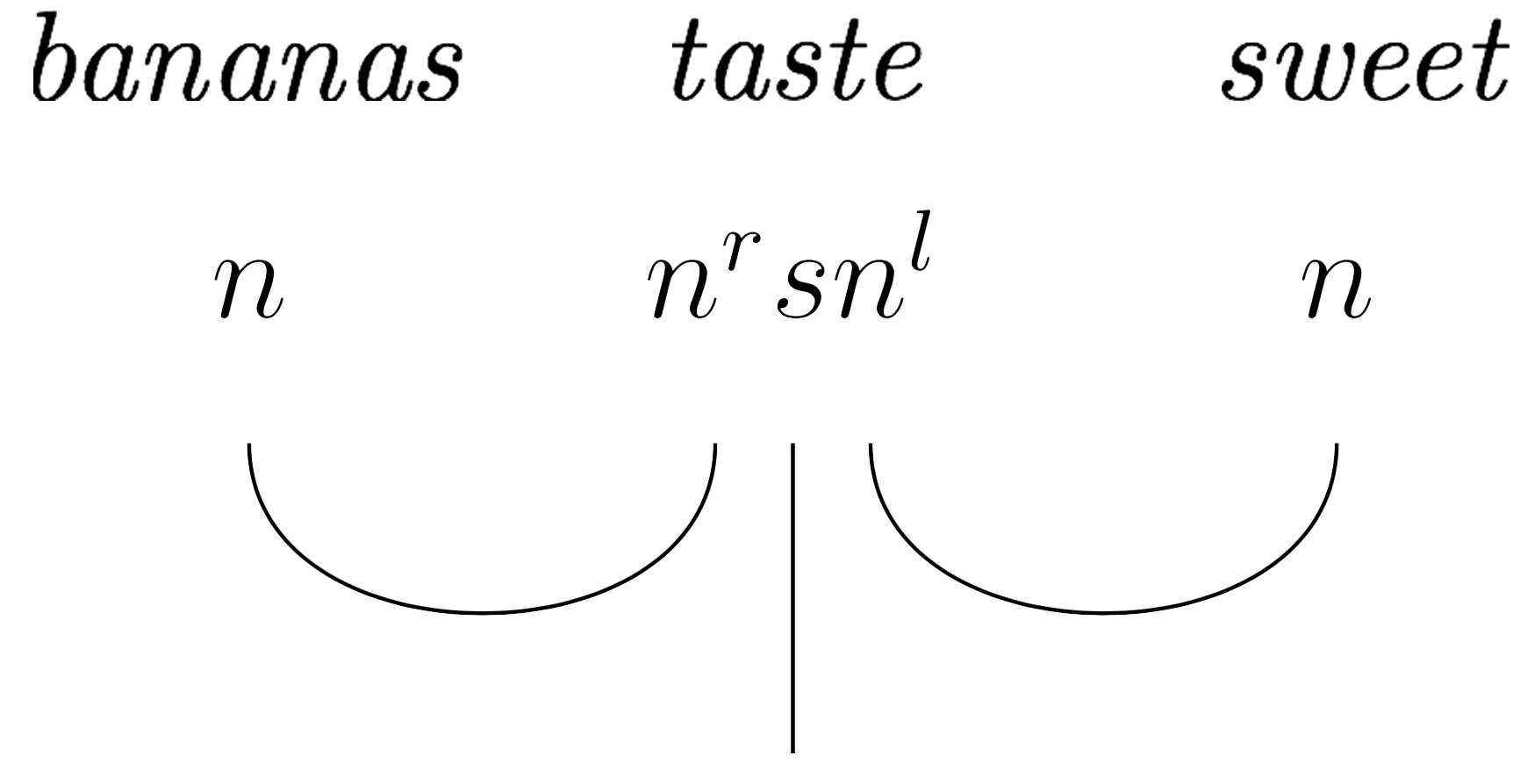
and each corresponds to a different conceptual space noun, n⇝Nsentence, s⇝Sverb, n rsn l⇝N⊗S⊗N\text{noun, }\; n \rightsquigarrow N \qquad\qquad \text{sentence, }\; s \rightsquigarrow S \qquad\qquad \text{verb, }\; n^r s n^l \rightsquigarrow N\otimes S \otimes N which we describe next.

Computing Meaning

The Noun Space NN

A noun is a state I→NI\to N, i.e. a convex subset of the noun space NN. Restricting our attention to food nouns, the space NN is a product of color, taste, and texture domains: N=N color⊗N taste⊗N texture⊂ℝ 8N=N_{\text{color}}\otimes N_{\text{taste}}\otimes N_{\text{texture}} \subset \mathbb{R}^8 where

• N colorN_{\text{color}} is the RGB color cube, i.e. the set of all triples (R,G,B)∈[0,1] 3(R,G,B)\in [0,1]^3.
• N tasteN_{\text{taste}} is the taste tetrahedron, i.e. the convex hull of four basic tastes: sweet, sour, bitter, and salty.
• N textureN_{\text{texture}} is the unit interval [0,1][0,1] where 0 represents liquid and 1 represents solid.

The noun banana is then a product of three convex subregions of NN:

That is, banana is the product of a yellow/green region, the convex hull of three points in the taste tetrahedron, and a subinterval of the texture interval. Other foods and beverages, avocados, chocolate, beer, etc. can be expressed similarly.

The Sentence Space SS

The meaning of a sentence is a convex subset of a sentence space SS. Here, SS is chosen as a simple-yet-sensible space to capture one’s experience when eating and drinking. It is the join semilattice on four points

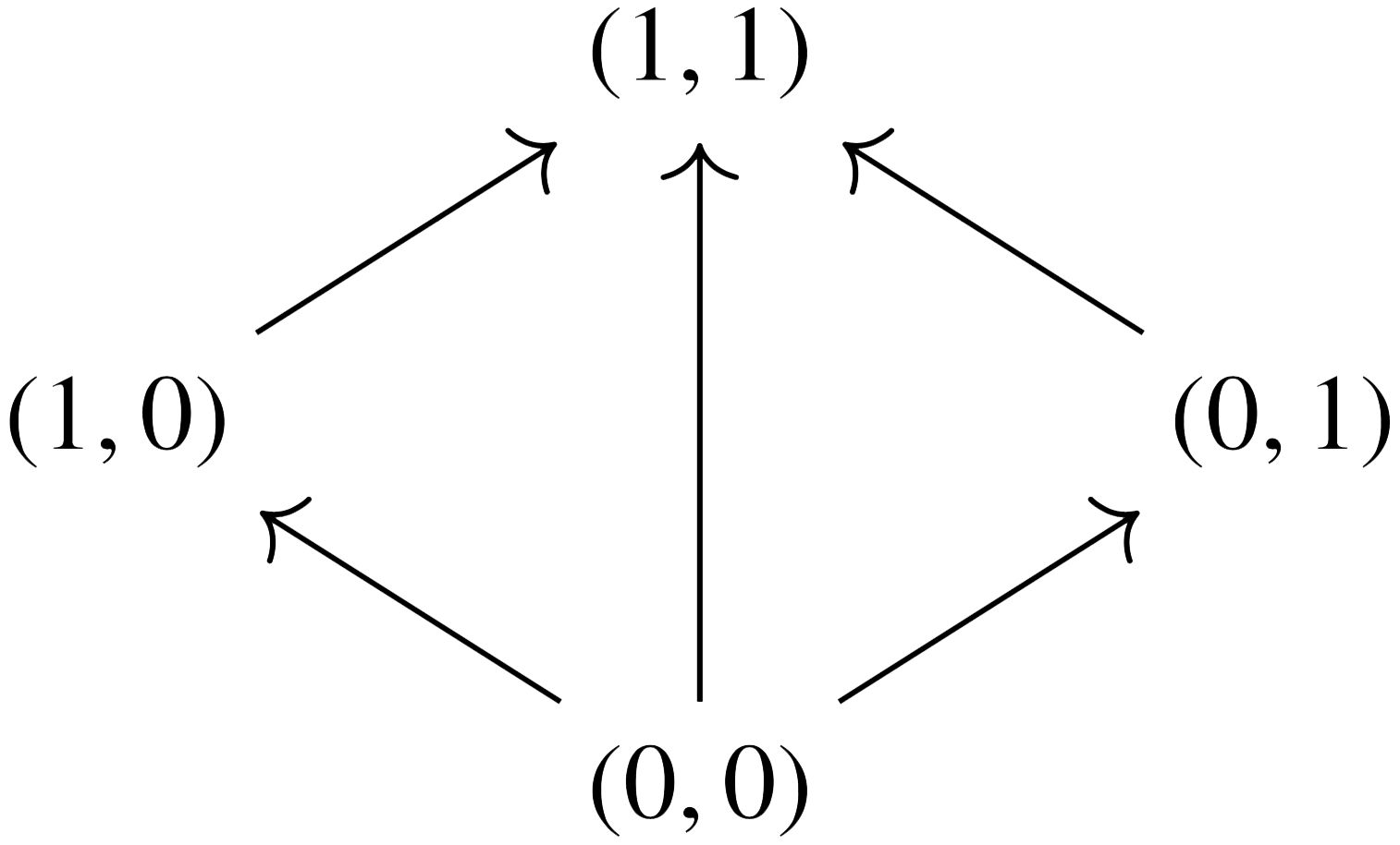
where in the first component, 0 = negative and 1 = positive, while in the second component, 0 = not surprising and 1 = surprising. For instance, (0,1)(0,1) represents negative and surprising while the convex subset {(1,1),(1,0)}\{(1,1),(1,0)\} represents positive.

The Verb Space N⊗S⊗NN\otimes S\otimes N

A transitive verb is a convex subset of N⊗S⊗NN\otimes S\otimes N. For instance, if we suppose momentarily that we live in a world in which one can survive on bananas and beer alone, then the verb taste can be represented by taste =Conv({greenbanana⊗{(0,0)}⊗bitter} ∪{greenbanana⊗{(1,1)}⊗sweet} ∪{yellowbanana⊗{(1,0)}⊗sweet} ∪{beer⊗{(0,1)}⊗sweet} ∪{beer⊗{(1,0)}⊗bitter}) \begin{aligned} t a s t e &= \text{Conv}( \{g r e e n\; b a n a n a \otimes\{(0,0)\}\otimes b i t t e r\}\\ &\,\cup \{g r e e n\; b a n a n a\otimes\{(1,1)\}\otimes s w e e t\}\\ &\,\cup \{y e l l o w\; b a n a n a\otimes\{(1,0)\}\otimes s w e e t\}\\ &\,\cup \{b e e r \otimes\{(0,1)\}\otimes s w e e t\}\\ &\,\cup \{b e e r\otimes\{(1,0)\}\otimes b i t t e r\}) \end{aligned} where Conv denotes the convex hull of the argument. Here, green is an intersective adjective, so green banana is computed by taking the intersection of the banana space with the green region of the color cube. Likewise for yellow banana.

Tying it all together

Finally, we compute the meaning of bananas taste sweet, which has grammar type reduction n(n rsn l)n≤(nn r)s≤s.n(n^r s n^l)n\leq (nn^r )s\leq s. In ConvexRel\mathsf{ConvexRel}, this corresponds to the following morphism: Nbananas⊗N⊗S⊗Ntaste⊗Nsweet⟶ϵ N⊗1 S⊗ϵ NS\overset{\text{bananas}}{N}\otimes\;\; \overset{\text{taste}}{N\;\; \otimes \;\; S\;\; \otimes \;\;N}\;\; \otimes \overset{\text{sweet}}{N}\;\;\;\overset{\epsilon_N\otimes 1_S\otimes\epsilon_N}{\longrightarrow}\;\;\; S bananastastesweet =(ϵ N⊗1 S⊗ϵ N)(bananas⊗taste⊗sweet) =(ϵ N⊗1 S)(banana⊗(greenbanana⊗{(1,1)} ∪yellowbanana⊗{(1,0)} ∪beer⊗{(0,1)})) ={(1,1),(1,0)} =positive \begin{aligned} b a n a n a s\; t a s t e\; s w e e t &= (\epsilon_N\otimes 1_S\otimes \epsilon_N)(b a n a n a s \otimes t a s t e \otimes s w e e t)\\ &=(\epsilon_N\otimes 1_S)(b a n a n a\otimes (g r e e n\; b a n a n a \otimes \{(1,1)\} \\ &\qquad\qquad\qquad\qquad\quad \cup y e l l o w\; b a n a n a \otimes\{(1,0)\} \\ &\qquad\qquad\qquad\qquad\quad \cup b e e r\otimes\{(0,1)\}))\\ &=\{(1,1),(1,0)\}\\ &= p o s i t i v e \end{aligned} Note that the rightmost ϵ N\epsilon_N selects subsets of the taste space that include sweet things and then deletes “sweet.” The leftmost ϵ N\epsilon_N selects subsets of the taste space that include banana and then deletes “banana.” We are left with a convex subset of SS, i.e. the meaning of the sentence.

Closing Remarks

Although not shown in the example above, one can also account for relative pronouns using certain morphisms called multi-wires or spiders (these arise from commutative special dagger Frobenius structures). The authors also give a toy example from the non-food world by modeling movement of a person from one location to another, using time and space to define new noun, sentence, and verb spaces.

In short, the conceptual spaces framework seeks to capture meaning in a way that resembles human thought more closely than the vector space model. This leaves us to puzzle over a couple of questions: 1) Do all concepts exhibit a convex structure? and 2) How might the conceptual spaces framework be implemented experimentally?

I have often seen competent mathematicians and logicians, outside our circle, making technically erroneous comments about the univalence axiom, in conversations, in talks, and even in public material, in journals or the web.

For some time I was a bit upset about this. But maybe this is our fault, by often trying to explain univalence only imprecisely, mixing the explanation of the models with the explanation of the underlying Martin-Löf type theory, with none of the two explained sufficiently precisely.

There are long, precise explanations such as the HoTT book, for example, or the various formalizations in Coq, Agda and Lean.

But perhaps we don’t have publicly available material with a self-contained, brief and complete formulation of univalence, so that interested mathematicians and logicians can try to contemplate the axiom in a fully defined form.

So here is an attempt of a  self-contained, brief and complete formulation of Voevodsky’s Univalence Axiom in the arxiv.

This has an Agda file with univalence defined from scratch as an ancillary file, without the use of any library at all, to try to show what the length of a self-contained definition of the univalence type is. Perhaps somebody should add a Coq “version from scratch” of this.

There is also a web version UnivalenceFromScratch to try to make this as accessible as possible, with the text and the Agda code together.

The above notes explain the univalence axiom only. Regarding its role, we recommend Dan Grayson’s introduction to univalent foundations for mathematicians.