At Compose, we work with developers who connect to our databases using a variety of languages and tools. One language that was recently requested by our developer community to cover is R. So, in this post, we will look at ways to connect to a Compose PostgreSQL deployment using R, and how we can run queries from our R development environment to Compose PostgreSQL.
The R language is an open source statistical language used mostly by data scientists, statisticians, and academics. One of the benefits of using R is that it is very good at data analysis. It provides you with powerful statistical and graphing tools, and it allows you to create and run data simulations. If you are not familiar with the language, you can head on over to Code School to try it out. Or, for the more inquisitive, you can download R here and try it. In addition to R, which comes with a simple IDE, I will be using RStudio. RStudio is a full-featured R IDE that you can download here and gives you the R console, an editor, and a history and debugging manager.
Connecting to Compose PostgreSQL
RPostgreSQL and RPostgres are two packages that will enable you to connect to PostgreSQL. RPostgreSQL is available on CRAN (Comprehensive R Archive Network) where the majority of R packages are archived. To download RPostgreSQL to your R development environment you run install.packages('RPostgreSQL'). On the other hand, RPostgres is not available on CRAN, so you first need to install R’s devtools with install.packages('devtools') and then install the package from Github. The instructions to download RPostgres are posted on their Github repository page.
Once you’ve downloaded the packages, you will notice that there is no difference in how they connect to PostgreSQL. Both use R's DBI package that provides a set of classes and methods that allow you to connect to databases such as PostgreSQL, MySQL, SQLite, and others. The following code shows you how to connect to Compose PostgreSQL using both RPostgreSQL and RPostgres.
# Connecting to RPostgreSQL

drv <- dbDriver('PostgreSQL')
db <- 'myDatabase'
host_db <- 'aws-us-east-1-portal.234.dblayer.com'
db_port <- '98939'
db_user <- 'henryviii'
db_password <- ‘happydays’

conn <- dbConnect(drv, dbname=db, host=host_db, port=db_port, user=db_user, password=db_password)

# Connecting to RPostgres
# with the same connection variables without 'drv'

conn <- dbConnect(RPostgres::Postgres(), dbname = db2, host=host_db, port=db_port, user=db_user, password=db_password)
After running conn, you know when you’ve established a connection to the database when no errors have been produced. Unless you write a custom function in R that indicates that you’ve successfully made a connection, you will not receive a confirmation that it's connected. One simple way to check if you have a connection, and to view the tables in your database, is to use either use dbListTables() to view all the tables, or dbExistsTable() to return a Boolean value if a specific table is found. That way you don’t have to write a custom function and you can use the methods that are available.
Preparing the Data
There are a few ways that we can insert data into a Compose PostgreSQL deployment. Either you can insert data via the terminal using psql, through the Compose UI, or through R’s development environment. Since we are concerned with using Compose PostgreSQL with R, let’s look at one way we could prepare our data, make a table, and insert it into our database using R.
First, let’s use a sample dataset provided by R: mtcars. This is the 1974 Motor Trend magazine car road test data. Although you probably will not use the datasets provided by R in any production database, they're useful if you want to practice inserting data and running queries for practice.
data('mtcars')
my_data <- data.frame(carname = rownames(mtcars), mtcars, row.names = NULL)
my_data$carname <- as.character(my_data$carname)
rm(mtcars)
The code above will set up our table as a data frame in R and rename the first column as carname, which has the list of cars, rather than the default row.name. If you don’t do this step, then row.name will be set as your column name when you upload it to PostgreSQL. After that, we remove mtcars rm(mtcars) from R’s development environment memory since we’ve stored it in the variable my_data.
Next, using the dbWriteTable method, we can write my_data to a PostgreSQL table. If the table hasn't been created, it will create one for us.
dbWriteTable(conn, name='cars', value=my_data)
To use it, we use the database connection variable we've created above conn, define a name for our table cars, and provide the data that should be written in the table that we also defined earlier as my_data. After you run it, take a look at your Compose PostgreSQL database. You will see that the table cars has been created and your data has been uploaded.
If your table already exists, even if it has no data in it, you will receive a warning message telling you that the process has been aborted. This safeguards you from rewriting data into a table that already exists. If you want to overwrite the table, however, then just set overwrite to TRUE within dbWriteTable.
dbWriteTable(conn, name='cars', value=my_data, overwrite=TRUE)
Now, when you look at your Compose database, you will find that it does not have a primary key set. You’ll want to do that now through a query.
Querying Data
There are two basic queries that we will use: dbGetQuery and dbSendQuery. While you might think that one is for getting data and the other is for sending data, this is not entirely the case. dbGetQuery will return all the query results in a data frame. dbSendQuery will register a request for your data then it has to be called by fetch for RPostgreSQL or dbFetch for RPostgres to receive the data. The fetch or dbFetch method allows you to set parameters to query your data in batches. For example, if you have a query that will return 10,000 items, you can assign a variable for the first 500 results a <- fetch(query, n = 500). Then you can create other variables for the rest of data using fetch by defining the number of results you want. If you use dbGetQuery you'd get all 10,000 queries, which might take a long time to process depending on the data retrieved.
Make sure that after your requests from dbSendQuery you call dbClearResult so that any pending queries from the database to your R environment are removed. dbGetQuery does this for you by implementing dbSendQuery, fetch, then dbClearResult behind the scenes. Also, make sure to disconnect dbDisconnect from the database once your query is done.
Going back to our Compose PostgreSQL primary key warning. Now that we know about how to make queries, we will go ahead and set a primary key in the cars table. To do this, we will write an SQL query and assign the primary key to the first column using the dbGetQuery method.
dbGetQuery(conn, 'ALTER TABLE cars ADD CONSTRAINT cars_pk PRIMARY KEY ("carnames");')
You could use dbSendQuery which would produce the same result, but for interactive queries, always use dbGetQuery. When setting up your table, you will also want to make sure to create indexes using dbGetQuery with the appropriate SQL syntax.
Another useful query method that will give us an overview of the data in our table is dbReadTable. This will send us the entire table. It is essentially the same as querying dbGetQuery(conn, ‘SELECT * FROM cars;’).
dbReadTable(conn, 'cars')
dbReadTable uses dbGetQuery in the background and just gives us an easy way to look at our data without writing the SQL command.
Creating queries to give us customized data is essentially the same as writing them in SQL. The difference is that your results are is stored as a variable in R. For example, if we wanted to get the cars that have at least a 6 cycle engine and at least 5 gears, our query would look like the following:
carQuery <- dbSendQuery(conn, 'select carname, cyl, gear from cars where cyl >= 6 and gear >= 5;')
result <- fetch(carQuery)
dbClearResult(carQuery)
The code above creates a variable called carQuery that contains our SQL query. Then we fetch the results of the query and save them in the variable results. If we do not set fetch to a variable, our results will not be saved and we will have to run the carQuery query again. After we've stored our data in results , we clear the query by inserting carQuery into the dbClearResult method.
If we look at the data stored within results, you will find the following:

Now that we have our results, we can choose to keep them within our R environment, or insert them into another table within our Compose PostgreSQL deployment. It really depends on what you’d like to do. If you want to store it back into your Compose database, then just write dbWriteTable(conn, 'my_new_table', results) and you'll have a new table my_new_table with your new data.
Refresh
So, we've covered some of the essential methods provided by RPostgreSQL and RPostgres. If you're familiar with SQL, then querying and modifying data will be easy since you create them using SQL syntax. I'd recommend looking at the documentation for RPostgreSQL and RPostgres, which will provide you with other methods that are available to query data from PostgreSQL to use with R. Overall, using R superpowers to analyze data from your own Compose PostgreSQL datasets, will provide you with the opportunity to take a deep dive into your data and crunch some serious numbers.


 Salamanca’s system was relatively low tech. That is to say you could not just walk up to a street terminal and use your credit card, but needed to go to an authorized location with fixed office hours where you could complete the registration. Between that complexity and the annual only fee, a conscious decision was made not to ride Salamanca’s bike-share.


 13-year-old Dayany dancing outside a housing project in Mott Haven. Photo by Taylor Lindsay
 Space near housing projects in the South Bronx. Photo by Taylor Lindsay
 Kids and adults outside housing projects in the South Bronx. Photo by Taylor Lindsay
 Mona, a member of Mitchell Houses Tenants Association, encourages interested participants to get involved with the project. Photo by Lucia della Paolera
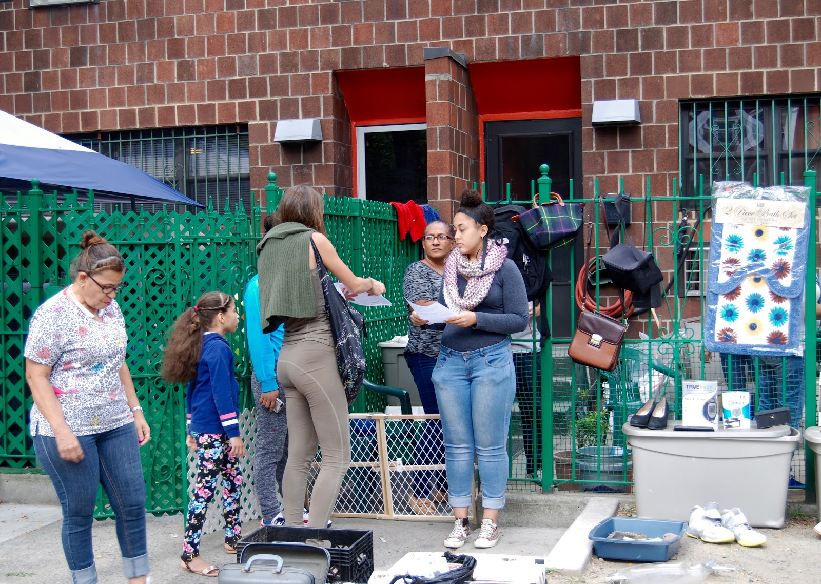
 Lucia della Paolera speaks to locals about the project. Photo by Taylor Lindsay
 Neighborhood resident Elijah, looking at a flyer for South Bronx Cribs. Photo by Taylor Lindsay
 Project Director Lucia della Paolera outside ID Studio in Mott Haven. Photo by Taylor Lindsay
 Lucia della Paolera speaks to locals about the project. Photo by Taylor Lindsay
 Lucia della Paolera speaks to locals about the project. Photo by Taylor Lindsay
 Trudy (22), a future participant in South Bronx Cribs. Photo by Taylor Lindsay
 Lucia della Paolera speaks to locals about the project. Photo by Taylor Lindsay